Batch Multiple Simulations Run

This RMarkdown file executes run type of batch simulation. The script utilizes the gastroPlusAPI package to communicate with the GastroPlus X 10.2 service. A batch simulation allows you to run multiple defined simulations for any number of compounds or scenarios.

The output from the batch simulation run is then used to create a Cp-time plot.

To customize your study with this script for a different simulation / project / variables, please make changes to the set-input-information code-chunk.

Configure required packages

Load other necessary packages(tidyverse) required to execute the data manipulation and visualization in the script
Load gastroPlusAPI package
Load gastroPlusRModuLens package

R

library(tidyverse)
library(gastroPlusAPI)
library(gastroPlusRModuLens)

# set default ggplot2 theme and options
theme_set(
  theme_gastroPlus_grid()
)
set_default_ggplot_options()

Set working directory

Set working directory as the current source editor context

R

if (rstudioapi::isAvailable()){
  current_working_directory <- dirname(rstudioapi::getSourceEditorContext()$path)
  setwd(current_working_directory)
}

Start GPX Service

Establishes a connection to the GastroPlus service, which allows R to communicate with GastroPlus through its API

R

gpx_service <- start_service(verbose=FALSE)

CODE

✔ Configured the GastroPlus Service

R

gpx_service$is_alive()

CODE

[1] TRUE

Setup Input Information

Make modification to the variables in this chunk to customize your workflow.

project_path: Location of the gpx project

simulation_name: Subset of simulation names to include in the run, or NULL to include all simulations

run_name: Name of the run that will be created

R

project_path <- "../../ProjectFiles/GPX Library.gpproject"

simulation_name <- NULL

run_name <- "BatchSimsRun"

Execute the Run

Based on the details mentioned in the previous code chunk, the batch simulation run will be created, executed and results will be shown

R

#Load the project
open_project(project_path)

if (is.null(simulation_name)) {
  simulation_name <- get_simulations()$simulation_name
}

#Create run and execute simulations
create_run(run_name = run_name, run_type = RunType$BatchSimulation)

add_simulations_to_run(run_name = run_name, simulation_names = simulation_name)

execute_run(run_name = run_name)

Process Run Output

This section retrieves and processes the results from the batch simulation run, including:

Getting summary output with pharmacokinetic parameters

Identifying and retrieving the concentration-time series data

Retrieving observed data for comparison

Build Series Descriptors

Series descriptors include the compound name and description of what is measured. Some series descriptors are defined by only the compound name and some StateType. Other series descriptors are defined by additional features, like CompartmentType.

The build_series_descriptors() function accepts one or more compound names along with one or more unnamed sets of series descriptors (without the compound name). For series descriptors that are defined by multiple features - like CompartmentType and StateType, wrap in c().

R

all_compounds <- unlist(get_project_assets("Compound")$assets)
all_compounds

CODE

[1] "Atenolol"            "Propranolol HCl"     "Ranitidine"         
[4] "Brick Dust"          "Piroxicam"           "Carbamazepine"      
[7] "Ketoprofen"          "Furosemide"          "Metoprolol Tartrate"

All series descriptors could be generated with one call to build_series_descriptors(), or certain series could grouped together for data manipulation purposes after collecting the data.

R

cp_series_descriptors <- build_series_descriptors(
  compound = all_compounds,
  c(CompartmentType$SystemicCirculation, StateType$ConcentrationPlasma),
  # Alternative: will check for venous return concentration (PBPK model)
  c(CompartmentType$VenousReturn, StateType$ConcentrationPlasma)
)

mass_series_descriptors <- build_series_descriptors(
  compound = all_compounds,
  StateType$TotalAbsorbed,
  StateType$TotalDissolved
)

series_descriptors <- c(
  cp_series_descriptors,
  mass_series_descriptors
)

Get Simulated Data

The functions get_series_data_project(), get_series_data_run(), and get_series_data_simulation() are all extensions of gastroPlusAPI::get_series_data() that operate on multiple runs, simulations, and series.

get_series_data_project() collects the desired series for the entire project, optionally subset to some values of run_name and/or simulation_name.
get_series_data_run() collects the desired series for one run, optionally subset to some values of simulation_name.
get_series_data_simulation() collects the desired series for one simulation in one run.

R

series_data <- get_series_data_run(
  run_name = run_name,
  series_descriptor = series_descriptors
)

glimpse(series_data)

CODE

Rows: 1,387
Columns: 10
$ run_name                        <chr> "BatchSimsRun", "BatchSimsRun", "Batch…
$ simulation_name                 <chr> "Atenolol 100mg PO tablet", "Atenolol …
$ series_name                     <chr> "Atenolol - Systemic Circulation - Con…
$ dependent_unit                  <chr> "ng/mL", "ng/mL", "ng/mL", "ng/mL", "n…
$ independent_unit                <chr> "h", "h", "h", "h", "h", "h", "h", "h"…
$ iteration                       <int> 0, 0, 0, 0, 0, 0, 0, 0, 0, 0, 0, 0, 0,…
$ dependent                       <dbl> 0.000000e+00, 2.651325e-16, 4.043352e-…
$ independent                     <dbl> 0.000000e+00, 2.217896e-06, 4.131786e-…
$ simulation_iteration_key_name   <chr> "Atenolol 100mg PO tablet \a0", "Ateno…
$ simulation_iteration_key_name_2 <chr> "Atenolol 100mg PO tablet", "Atenolol …

R

series_data %>%
  count(series_name, independent_unit, dependent_unit)

CODE

# A tibble: 27 × 4
   series_name                             independent_unit dependent_unit     n
   <chr>                                   <chr>            <chr>          <int>
 1 Atenolol - Systemic Circulation - Conc… h                ng/mL             50
 2 Atenolol - Total Absorbed               h                mg                50
 3 Atenolol - Total Dissolved              h                mg                50
 4 Brick Dust - Systemic Circulation - Co… h                ng/mL             28
 5 Brick Dust - Total Absorbed             h                mg                28
 6 Brick Dust - Total Dissolved            h                mg                28
 7 Carbamazepine - Systemic Circulation -… h                ng/mL             49
 8 Carbamazepine - Total Absorbed          h                mg                49
 9 Carbamazepine - Total Dissolved         h                mg                49
10 Furosemide - Systemic Circulation - Co… h                ng/mL             60
# ℹ 17 more rows

R

series_data %>%
  count(run_name, simulation_name)

CODE

# A tibble: 9 × 3
  run_name     simulation_name                         n
  <chr>        <chr>                               <int>
1 BatchSimsRun Atenolol 100mg PO tablet              150
2 BatchSimsRun Brick Dust 10mg PO tablet              84
3 BatchSimsRun Carbamazepine 200mg PO tablet         147
4 BatchSimsRun Furosemide 40mg PO tablet             180
5 BatchSimsRun Ketoprofen 100mg PO tablet            171
6 BatchSimsRun Metoprolol Tartrate 200mg PO tablet   179
7 BatchSimsRun Piroxicam 20mg PO capsule             143
8 BatchSimsRun Propranolol HCl 160mg PO tablet       174
9 BatchSimsRun Ranitidine 150mg PO tablet            159

Get Observed Data

The get_observed_series_data() function is an extension of gastroPlusAPI::get_observed_series() that operates on any subset of group_name, group_type, series_name, and/or series_type and always returns a data frame. When called with no arguments, get_observed_series_data() collects all observed data in the open project. This function also calculates standard deviation (std_dev) derived from reported mean and CV%.

R

observed_data_inventory <- get_experimental_data_inventory()
observed_data_inventory

CODE

# A tibble: 6 × 4
  group_name                     group_type   series_name            series_type
  <chr>                          <chr>        <chr>                  <chr>      
1 Ketoprofen Solubility          Solubility   Solubility vs pH       pH_Solubil…
2 Propranolol HCl Solubility     Solubility   Solubility vs pH       pH_Solubil…
3 Piroxicam Solubility           Solubility   Solubility vs pH       pH_Solubil…
4 Piroxicam PO Cp time           ExposureData Piroxicam Exposure Pl… UncertainC…
5 Propranolol HCl PO Cp time     ExposureData Propranolol HCl Expos… UncertainC…
6 Metoprolol Tartrate PO Cp time ExposureData Metoprolol Tartrate E… UncertainC…

R

observed_data <- get_observed_series_data()
observed_exposure_data <- observed_data %>% 
  filter(group_type == "ExposureData")
observed_solubility_data <- observed_data %>% 
  filter(group_type == "Solubility")

glimpse(observed_exposure_data)

CODE

Rows: 30
Columns: 20
$ group_name             <chr> "Piroxicam PO Cp time", "Piroxicam PO Cp time",…
$ group_type             <chr> "ExposureData", "ExposureData", "ExposureData",…
$ series_name            <chr> "Piroxicam Exposure Plasma", "Piroxicam Exposur…
$ series_type            <chr> "UncertainConcentrationSeries", "UncertainConce…
$ independent_unit       <chr> "h", "h", "h", "h", "h", "h", "h", "h", "h", "h…
$ dependent_unit         <chr> "ng/mL", "ng/mL", "ng/mL", "ng/mL", "ng/mL", "n…
$ independent            <dbl> 0.0, 0.5, 1.0, 2.0, 3.0, 6.0, 12.0, 24.0, 48.0,…
$ dependent              <dbl> 0.0, 31.4, 933.9, 2507.6, 2609.4, 2112.4, 1774.…
$ module                 <chr> "SystemicCirculation", "SystemicCirculation", "…
$ section                <chr> "", "", "", "", "", "", "", "", "", "", "", "",…
$ compartment            <chr> "SystemicCirculation", "SystemicCirculation", "…
$ state                  <chr> "ConcentrationPlasma", "ConcentrationPlasma", "…
$ dose                   <dbl> 0.0200, 0.0200, 0.0200, 0.0200, 0.0200, 0.0200,…
$ dose_unit              <chr> "g", "g", "g", "g", "g", "g", "g", "g", "g", "g…
$ infusion_time          <int> 0, 0, 0, 0, 0, 0, 0, 0, 0, 0, 0, 0, 0, 0, 0, 0,…
$ infusion_time_unit     <chr> "s", "s", "s", "s", "s", "s", "s", "s", "s", "s…
$ body_mass              <int> 0, 0, 0, 0, 0, 0, 0, 0, 0, 0, 0, 0, 0, 74000, 7…
$ body_mass_unit         <chr> "g", "g", "g", "g", "g", "g", "g", "g", "g", "g…
$ uncertainty_percentage <dbl> 0.0, 0.0, 0.0, 0.0, 0.0, 0.0, 0.0, 0.0, 0.0, 0.…
$ std_dev                <dbl> 0.0000, 0.0000, 0.0000, 0.0000, 0.0000, 0.0000,…

R

observed_exposure_data %>%
  count(series_name, series_type)

CODE

# A tibble: 3 × 3
  series_name                         series_type                      n
  <chr>                               <chr>                        <int>
1 Metoprolol Tartrate Exposure Plasma UncertainConcentrationSeries     9
2 Piroxicam Exposure Plasma           UncertainConcentrationSeries    13
3 Propranolol HCl Exposure Plasma     UncertainConcentrationSeries     8

Plot Results

Define common values across simulated and observed data

Since the names of runs, simulations, and observed series are user-defined, the shared variable names in simulated and observed data will not always match and may require some data manipulation.

In many projects, even though both series_data and observed_data include the series_name variable, but the content of this variable is not always well aligned.

R

intersect(names(series_data), names(observed_exposure_data))

CODE

[1] "series_name"      "dependent_unit"   "independent_unit" "dependent"       
[5] "independent"

R

series_data %>% 
  count(series_name, independent_unit, dependent_unit)

CODE

# A tibble: 27 × 4
   series_name                             independent_unit dependent_unit     n
   <chr>                                   <chr>            <chr>          <int>
 1 Atenolol - Systemic Circulation - Conc… h                ng/mL             50
 2 Atenolol - Total Absorbed               h                mg                50
 3 Atenolol - Total Dissolved              h                mg                50
 4 Brick Dust - Systemic Circulation - Co… h                ng/mL             28
 5 Brick Dust - Total Absorbed             h                mg                28
 6 Brick Dust - Total Dissolved            h                mg                28
 7 Carbamazepine - Systemic Circulation -… h                ng/mL             49
 8 Carbamazepine - Total Absorbed          h                mg                49
 9 Carbamazepine - Total Dissolved         h                mg                49
10 Furosemide - Systemic Circulation - Co… h                ng/mL             60
# ℹ 17 more rows

R

observed_exposure_data %>% 
  count(series_name, independent_unit, dependent_unit)

CODE

# A tibble: 3 × 4
  series_name                         independent_unit dependent_unit     n
  <chr>                               <chr>            <chr>          <int>
1 Metoprolol Tartrate Exposure Plasma h                ng/mL              9
2 Piroxicam Exposure Plasma           h                ng/mL             13
3 Propranolol HCl Exposure Plasma     h                ng/mL              8

The desired content to align simulated and observed data might exist in other variables.

R

setdiff(names(series_data), names(observed_exposure_data))

CODE

[1] "run_name"                        "simulation_name"                
[3] "iteration"                       "simulation_iteration_key_name"  
[5] "simulation_iteration_key_name_2"

R

series_data %>% 
  count(run_name, simulation_name)

CODE

# A tibble: 9 × 3
  run_name     simulation_name                         n
  <chr>        <chr>                               <int>
1 BatchSimsRun Atenolol 100mg PO tablet              150
2 BatchSimsRun Brick Dust 10mg PO tablet              84
3 BatchSimsRun Carbamazepine 200mg PO tablet         147
4 BatchSimsRun Furosemide 40mg PO tablet             180
5 BatchSimsRun Ketoprofen 100mg PO tablet            171
6 BatchSimsRun Metoprolol Tartrate 200mg PO tablet   179
7 BatchSimsRun Piroxicam 20mg PO capsule             143
8 BatchSimsRun Propranolol HCl 160mg PO tablet       174
9 BatchSimsRun Ranitidine 150mg PO tablet            159

R

setdiff(names(observed_exposure_data), names(series_data))

CODE

 [1] "group_name"             "group_type"             "series_type"           
 [4] "module"                 "section"                "compartment"           
 [7] "state"                  "dose"                   "dose_unit"             
[10] "infusion_time"          "infusion_time_unit"     "body_mass"             
[13] "body_mass_unit"         "uncertainty_percentage" "std_dev"

R

observed_exposure_data %>% 
  count(series_type)

CODE

# A tibble: 1 × 2
  series_type                      n
  <chr>                        <int>
1 UncertainConcentrationSeries    30

Aligning the most important features of simulated and observed data will produce the most meaningful visualizations.

R

series_data <- series_data %>% 
  mutate(
    category = case_when(
      series_name %in% cp_series_descriptors ~ "Concentration",
      series_name %in% mass_series_descriptors ~ "Mass"
    ),
    
    endpoint = str_remove(series_name, "^[^-]*-\\s?"),
    
    compound = trimws(str_replace(series_name, "(^[^-]*)?-.*", "\\1"))
  )

series_data %>% 
  count(category, endpoint, compound)

CODE

# A tibble: 27 × 4
   category      endpoint                                    compound          n
   <chr>         <chr>                                       <chr>         <int>
 1 Concentration Systemic Circulation - Concentration Plasma Atenolol         50
 2 Concentration Systemic Circulation - Concentration Plasma Brick Dust       28
 3 Concentration Systemic Circulation - Concentration Plasma Carbamazepine    49
 4 Concentration Systemic Circulation - Concentration Plasma Furosemide       60
 5 Concentration Systemic Circulation - Concentration Plasma Ketoprofen       57
 6 Concentration Systemic Circulation - Concentration Plasma Metoprolol T…    65
 7 Concentration Systemic Circulation - Concentration Plasma Piroxicam        55
 8 Concentration Systemic Circulation - Concentration Plasma Propranolol …    62
 9 Concentration Systemic Circulation - Concentration Plasma Ranitidine       53
10 Mass          Total Absorbed                              Atenolol         50
# ℹ 17 more rows

R

observed_exposure_data <- observed_exposure_data %>% 
  mutate(
    category = "Concentration",
    endpoint = "Systemic Circulation - Concentration Plasma",
    compound = trimws(str_remove(series_name, "Exposure Plasma"))
  )

observed_exposure_data %>% 
  count(category, endpoint, compound, dose, dose_unit)

CODE

# A tibble: 3 × 6
  category      endpoint                          compound  dose dose_unit     n
  <chr>         <chr>                             <chr>    <dbl> <chr>     <int>
1 Concentration Systemic Circulation - Concentra… Metopro… 0.156 g             9
2 Concentration Systemic Circulation - Concentra… Piroxic… 0.02  g            13
3 Concentration Systemic Circulation - Concentra… Propran… 0.140 g             8

R

# subset of simulated data including concentration data.
cp_series_data <- series_data %>% 
  filter(
    category == "Concentration"
  )

cp_series_data %>% 
  count(category, endpoint, compound)

CODE

# A tibble: 9 × 4
  category      endpoint                                    compound           n
  <chr>         <chr>                                       <chr>          <int>
1 Concentration Systemic Circulation - Concentration Plasma Atenolol          50
2 Concentration Systemic Circulation - Concentration Plasma Brick Dust        28
3 Concentration Systemic Circulation - Concentration Plasma Carbamazepine     49
4 Concentration Systemic Circulation - Concentration Plasma Furosemide        60
5 Concentration Systemic Circulation - Concentration Plasma Ketoprofen        57
6 Concentration Systemic Circulation - Concentration Plasma Metoprolol Ta…    65
7 Concentration Systemic Circulation - Concentration Plasma Piroxicam         55
8 Concentration Systemic Circulation - Concentration Plasma Propranolol H…    62
9 Concentration Systemic Circulation - Concentration Plasma Ranitidine        53

Concentration vs Time

R

cp_plot_list <- unique(cp_series_data$compound) %>% 
  map(function(.compound) {
    cp_series_subset <- cp_series_data %>% 
      filter(compound == .compound)
    
    observed_exposure_subset <- observed_exposure_data %>% 
      filter(compound == .compound)
    
    plot_series_data(
      data_sim = cp_series_subset,
      data_obs = observed_exposure_subset,
      x_label = "Time (h)",
      y_label = "Concentration (ng/mL)",
    ) +  
      labs(
        subtitle = .compound
      )
  })
ggpubr::ggarrange(plotlist = cp_plot_list)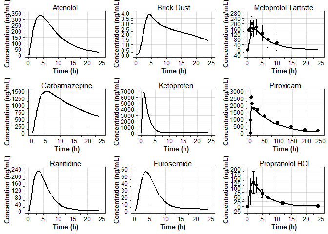

Concentration and Mass vs Time

When data with 2 unique values of dependent_unit is provided to plot_series_data(), a dual-axis is created.

R

# concentration and mass-time curves (dual axis).
cp_mass_plot_list <- unique(series_data$compound) %>% 
  map(function(.compound) {
    series_subset <- series_data %>% 
      filter(compound == .compound)
    
    plot_series_data(
      series_subset,
      color = endpoint,
      linetype = category,
      x_label = "Time (h)",
      y_label = "Concentration\n(ng/mL)",
      y2_label = "Mass (mg)"
    ) +  
      labs(
        subtitle = .compound,
        color = NULL,
        linetype = NULL
      ) + 
      guides(
        color = guide_legend(NULL)
      )
  })
ggpubr::ggarrange(plotlist = cp_mass_plot_list, common.legend = TRUE)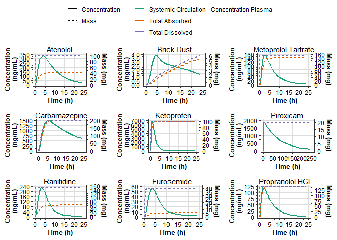

Solubility Observed Data

R

plot_series_data(
  data_obs = observed_solubility_data,
  x_label = "pH",
  y_label = "Solubility (ng/mL)",
) + 
  scale_y_continuous() + 
  facet_wrap(~ group_name, scales = "free_y")

CODE

Scale for y is already present.
Adding another scale for y, which will replace the existing scale.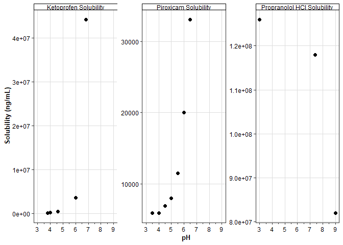

Diagnostic plots

With observed and predicted data available, we can also plot observed vs predicted values or residuals vs predicted values.

Observed vs Predicted

R

intersect(names(observed_exposure_data), names(cp_series_data))

CODE

[1] "series_name"      "independent_unit" "dependent_unit"   "independent"     
[5] "dependent"        "category"         "endpoint"         "compound"

R

# combine observed and simulated data.
data_obs_pred <- cp_series_data %>% 
  select(-c(series_name)) %>% 
  rename(Predicted = dependent) %>% 
  # inner join to only keep the rows with matching by variables.
  inner_join(
    observed_exposure_data %>% 
      select(-c(series_name)) %>% 
      rename(Observed = dependent),
    by = join_by(
      independent_unit, dependent_unit, independent, endpoint, category, compound
    )
  ) %>% 
  mutate(
    Residuals = Observed - Predicted
  )

plot_obs_vs_pred(
  data = data_obs_pred,
  obs = Observed,
  pred = Predicted,
) + 
  facet_wrap(~ compound)

CODE

Warning in scale_x_continuous(..., transform = transform_log10()): log-10
transformation introduced infinite values.

CODE

Warning in scale_y_continuous(..., transform = transform_log10()): log-10
transformation introduced infinite values.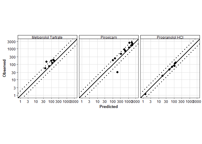

Residuals vs Predicted

R

plot_res_vs_pred(
  data = data_obs_pred,
  res = Residuals,
  pred = Predicted
) + 
  scale_x_continuous() + 
  scale_y_continuous() + 
  facet_wrap(~ compound, scales = "free")

CODE

Scale for x is already present.
Adding another scale for x, which will replace the existing scale.
Scale for y is already present.
Adding another scale for y, which will replace the existing scale.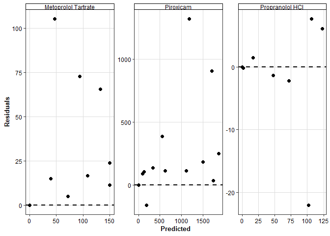

Kill GPX Service

R

gpx_service$kill()

CODE

[1] TRUE