Perform Global Sensitivity Analysis using Morris Method

This RMarkdown file creates and executes PSA run with user-defined set of variables data points. The script utilizes the gastroPlusAPI package to communicate with the GastroPlus X 10.2 service. It demonstrates how to perform a global sensitivity analysis (GSA) using the Morris method (also known as Elementary Effects method) with GastroPlus. The script identifies which input variables have the greatest influence on model outputs, helping to prioritize further investigations and optimize model development.

The Morris method is particularly effective for PBPK models with numerous input parameters and non-linear behaviors. It systematically perturbs one input at a time across multiple trajectories, calculating elementary effects to estimate:

μ*: the mean absolute effect, indicating overall parameter influence.

σ: the standard deviation, reflecting non-linearity and interactions.

This approach requires fewer model evaluations than variance-based methods, making it suitable for complex PBPK models.Studies have shown that the Morris method can effectively identify influential parameters, aiding in model simplification and optimization ([@ROBINS2024106881, @McNally_2011]) .

To customize your study with this script for a different simulation / project / variables, please make changes to the “Set Input Information” section.

Configure required packages

Load other necessary packages required to execute the script (tidyverse, plotly,corrplot and sensitivity)
Load gastroPlusAPI package

R

library(tidyverse)
library(gastroPlusAPI)
library(plotly)
library(corrplot)
library(sensitivity)

Set working directory

Set working directory as the current source editor context

R

if (rstudioapi::isAvailable()){
  current_working_directory <- dirname(rstudioapi::getSourceEditorContext()$path)
  setwd(current_working_directory)
}

Start GPX Service

Establishes a connection to the GastroPlus service, which allows R to communicate with GastroPlus through its API

R

gpx_service <- start_service(verbose=FALSE)

CODE

✔ Configured the GastroPlus Service

R

gpx_service$is_alive()

CODE

[1] TRUE

Setup Input Information

Open an existing GastroPlus project,create a PSA run named global_sensitivity_analysis. Specify variables to include in the sensitivity analysis (variable_names). Defines upper and lower bounds for each parameter based on domain knowledge or default scaling. Prepare a data frame (psa_parameters_df) used to sample parameter space via Morris method.

Make modification to the variables in this chunk to customize your analysis.

project_path: Location of the project where PSA run will be created

simulation_name: Name of the simulation for the PSA run

run_name: Name of the PSA run that will be created

Create a run in GPX to utilize the values provided by morris method and retrieve corresponding output for further analysis (next section)

Variables required for Morris method (refer morris method from sensitivity package):

num_of_repetition_per_factor: Number of elementary effects computed per factor / variable
num_of_levels: Number of levels of the OAT (One-At-a-Time) design. Higher values give finer resolution but increase computational cost

variable_names: Vector/list containing the variable information required to setup the PSA run in GPX project. Variable names can be obtained after opening the project (open_project function) and then calling the get_variables function

variable_information: Vector/list containing the variable information where the variable_names of the parameters on which the GSA is defined

psa_parameters_df: define the upper and lower bound of the GSA, in the case the bounds are specific pass them directly to the variable name as seen for “Stomach | Lumen | pH” otherwise, set the lower and uper bound to the baseline values of the parameters as seen for other parameters. The variable bounds will be used to generate the set of points to be sampled in the design space

output_variable: The model output variable whose sensitivity to input is to be calculated (possible values are “cmax”, “tmax”, absorbed”, “bioavailable”, “portal_vein” “infinite_exposure”, “total_exposure”, liver_cmax” )

R

project_path = "../../ProjectFiles/GPX Library.gpproject"
simulation_name = "Atenolol 100mg PO tablet"
run_name = "global_sensitivity_analysis"
open_project(project_path)

#Create new PSA run
create_run(run_name, RunType$ParameterSensitivityAnalysis)

#Add simulations to the run
add_simulations_to_run(run_name, c(simulation_name))
# confirm that the simulation was added to the run.
get_simulations_in_run(run_name)

CODE

[[1]]
[1] "Atenolol 100mg PO tablet"

R

variable_names = c("Stomach | Lumen | pH",
                   "Small Intestine Transit Time",
                   "Ileum1 | Surface Area Enhancement Factor",
                   "Stomach | Transit Time",
                   "Small Intestine Length",
                   "Solubility",
                   "Particle | Density")

variable_information <- get_variable_information(
  run_name = run_name, 
  simulation_name = simulation_name, 
  variable_names = variable_names
)

glimpse(variable_information)

CODE

Rows: 7
Columns: 4
$ input_variable_name <chr> "Ileum1 | Surface Area Enhancement Factor", "Parti…
$ scalar_type         <chr> "Unitless", "Concentration", "Length", "Time", "Co…
$ variable_name       <chr> "pharma::PhysiologyRegimen-78kg HumanFasted Physio…
$ variable_value      <df[,2]> <data.frame[7 x 2]>

R

variable_information <- variable_information %>%
  unnest(cols = variable_value)

#define the upper and lower bound of the GSA, in the case the bounds are specific pass them directly to the variable name as seen for "Stomach | Lumen | pH" otherwise, set the lower and upper bound to the baseline values of the parameters as seen for other parameters. 
psa_parameters_df <- variable_information %>%
  transmute(
    variable_name = input_variable_name,
    baseline_value = value,
    lower_bound = case_when(
      variable_name == "Stomach | Lumen | pH" ~ 0.1 ,
      TRUE ~ 0.25 * baseline_value
    ),
    upper_bound = case_when(
      variable_name == "Stomach | Lumen | pH" ~ 3,
      TRUE ~ 1.75 * baseline_value
    ),
    unit = unit,
    scalar_type = scalar_type
  )


#Define parameters for morris GSA 
num_of_repetition_per_factor <- 20
num_of_levels <- 25

output_variable <- "absorbed"

cli::cli_alert_info("Specified input information is as follows")

CODE

ℹ Specified input information is as follows

R

glimpse(variable_information)

CODE

Rows: 7
Columns: 5
$ input_variable_name <chr> "Ileum1 | Surface Area Enhancement Factor", "Parti…
$ scalar_type         <chr> "Unitless", "Concentration", "Length", "Time", "Co…
$ variable_name       <chr> "pharma::PhysiologyRegimen-78kg HumanFasted Physio…
$ unit                <chr> "[no units]", "g/mL", "m", "s", "g/m³", "[no units…
$ value               <dbl> 3.029, 1.200, 3.250, 11880.000, 27000.000, 1.300, …

Configure Global Sensitvity Analysis to generate design matrix

Based on the variable input information provided, morris method will sample the datapoints for each variable specified. The code uses the morris() function from the R sensitivity package to sample the input space with One-At-a-Time (OAT) perturbations, create a design matrix containing parameter values for each parameter in the simulation. The design follows an OAT approach where one parameter changes at a time along trajectory.

R

# Morris method will generate the design matrix
morris_results <- morris(
  model = NULL, 
  factors = psa_parameters_df$variable_name, 
  r = num_of_repetition_per_factor,  # of trajectories
  design = list(type = "oat", levels = num_of_levels, grid.jump = floor(num_of_levels/2)),  
  binf = psa_parameters_df$lower_bound, 
  bsup = psa_parameters_df$upper_bound,
  scale = TRUE
)

design_matrix <- as_tibble(morris_results$X)

#Determine number of user defined simulations 
number_of_user_defined_simulations <- nrow(design_matrix)

cli::cli_alert_info(
    "{number_of_user_defined_simulations} simulations will be executed as part of the PSA run in GPX to determine the elementary effects of input variables on output variable")

CODE

ℹ 160 simulations will be executed as part of the PSA run in GPX to determine the elementary effects of input variables on output variable

Run the simulations in GPX

Utilize the values provided by morris method to the PSA configuration using user-defined values, and link the design matrix to GastroPlus input variables.Configure and execute the run to retrieve corresponding output for further analysis.

R

#Setup PSA Parameters List
psa_parameter_list <- list()
count = 1

for(var in psa_parameters_df$variable_name){
  var_info <- variable_information %>% filter(input_variable_name == var) 
  
  input_info <- psa_parameters_df %>% filter(variable_name == var) 
  
  scalar_values_list <- list()
  
  design_matrix_variable_values <- design_matrix %>% pull(var)
  
  i=1
  for(value in design_matrix_variable_values) {
    scalar_value <- ScalarValue$new(value, input_info$unit)
    scalar_values_list[[i]] <- scalar_value
    i = i+1
  }
  
  psa_parameter_list[[count]] <- PSAParameter$new(
    variable_name = var,
    baseline_value = var_info$value,
    unit = input_info$unit,
    scalar_type = var_info$scalar_type,
    number_of_tests = number_of_user_defined_simulations,
    user_defined_values = scalar_values_list
  )
  
  count = count + 1
}


#Setup PSA Setting
psa_setting <- PSASetting$new(
  analysis_mode = ParameterSensitivityAnalysisMode$UserDefined,
  simulate_baseline = FALSE,
  update_Kp = FALSE,
  number_of_user_defined_simulations = number_of_user_defined_simulations)

#Create PSA Configuration object
PSA_configuration <- PSAConfiguration$new(PSA_Setting = psa_setting,
                                          PSA_Parameters = psa_parameter_list)

#Create Run Configuration object
run_configuration <- RunConfiguration$new(PSA_Configuration = PSA_configuration)

#Configure the run in GPX
configure_run(run_name, run_configuration, use_full_variable_name = FALSE)

#Execute Run
execute_run(run_name)

Compile Run Output for analysis

Retrieve simulation output summaries from GastroPlus (get_simulation_keys() and get_summary_output()). Get the values for the variables in simulation iterations present in the run (get_iteration_records()). Produce a unified data frame for GSA analysis.

R

simulation_keys <- get_simulation_keys(run_name)

summary_output <- get_summary_output(run_name, simulation_keys$simulation_iteration_key_name) 

summary_output_variable_names <- colnames(summary_output)
summary_output$simulation_iteration_key <- simulation_keys$simulation_iteration_key_name

iteration_records <- get_iteration_records(run_name, unlist(simulation_keys$simulation_iteration_key_name), variable_information$input_variable_name)

#Re-structure iteration records so that it can be merged with summary output
iteration_records <- iteration_records %>% 
  tidyr::unnest(cols = where(is.list)) %>%
  tidyr::pivot_wider(id_cols=simulation_iteration_key, 
                     names_from=variable,
                     values_from=variable_value)

#Merge the two tibbles
input_output_merged <- dplyr::full_join(iteration_records, summary_output, by="simulation_iteration_key") %>% 
  unnest(cols=all_of(summary_output_variable_names), names_sep= " ") %>%
  unnest(cols=all_of(unlist(variable_information$input_variable_name)), names_sep=" ") 

glimpse(input_output_merged)

CODE

Rows: 160
Columns: 37
$ simulation_iteration_key                         <chr> "Atenolol 100mg PO ta…
$ `Ileum1 | Surface Area Enhancement Factor unit`  <chr> "[no units]", "[no un…
$ `Ileum1 | Surface Area Enhancement Factor value` <dbl> 0.9466, 0.9466, 3.218…
$ `Particle | Density unit`                        <chr> "g/m³", "g/m³", "g/m³…
$ `Particle | Density value`                       <dbl> 1350000, 1350000, 135…
$ `Small Intestine Length unit`                    <chr> "m", "m", "m", "m", "…
$ `Small Intestine Length value`                   <dbl> 3.4531, 3.4531, 3.453…
$ `Small Intestine Transit Time unit`              <chr> "s", "s", "s", "s", "…
$ `Small Intestine Transit Time value`             <dbl> 8910.0, 17820.0, 1782…
$ `Solubility unit`                                <chr> "g/m³", "g/m³", "g/m³…
$ `Solubility value`                               <dbl> 27000.0, 27000.0, 270…
$ `Stomach | Lumen | pH unit`                      <chr> "[no units]", "[no un…
$ `Stomach | Lumen | pH value`                     <dbl> 0.3417, 0.3417, 0.341…
$ `Stomach | Transit Time unit`                    <chr> "s", "s", "s", "s", "…
$ `Stomach | Transit Time value`                   <dbl> 1575, 1575, 1575, 157…
$ absorbed                                         <dbl> 0.3094681, 0.5026083,…
$ bioavailable                                     <dbl> 0.2983507, 0.4920607,…
$ `clearance unit`                                 <chr> "L/h", "L/h", "L/h", …
$ `clearance value`                                <dbl> 37.01235, 22.50756, 2…
$ `cmax unit`                                      <chr> "ng/mL", "ng/mL", "ng…
$ `cmax value`                                     <dbl> 256.7865, 374.1147, 4…
$ compound                                         <chr> "Atenolol", "Atenolol…
$ `infinite_exposure unit`                         <chr> "(ng/mL)*h", "(ng/mL)…
$ `infinite_exposure value`                        <dbl> 2701.801, 4442.952, 4…
$ iteration                                        <int> 0, 1, 2, 3, 4, 5, 6, …
$ `liver_cmax unit`                                <chr> "ng/mL", "ng/mL", "ng…
$ `liver_cmax value`                               <dbl> 296.2553, 423.8012, 4…
$ portal_vein                                      <dbl> 0.2983507, 0.4920607,…
$ run_simulation_iteration_key                     <chr> "global_sensitivity_a…
$ simulation_iteration_key_name                    <chr> "Atenolol 100mg PO ta…
$ simulation_iteration_key_name_2                  <chr> "Atenolol 100mg PO ta…
$ `tmax unit`                                      <chr> "h", "h", "h", "h", "…
$ `tmax value`                                     <dbl> 3.709168, 4.517222, 4…
$ `total_dose unit`                                <chr> "mg", "mg", "mg", "mg…
$ `total_dose value`                               <dbl> 100, 100, 100, 100, 1…
$ `total_exposure unit`                            <chr> "(ng/mL)*h", "(ng/mL)…
$ `total_exposure value`                           <dbl> 2581.972, 4229.401, 4…

Get Morris sensitivity analysis results

Get and plot GSA results from Morris method.

A higher mean (mu.star) indicates that the parameter has a higher influence on the output of the model, while a higher standard deviation (sigma) indicates higher interaction of the parameter with other parameters

R

if (output_variable %in% colnames(input_output_merged)) {
  output_values <- input_output_merged %>% pull(output_variable)
} else {
  column_of_interest <- paste(output_variable, "value", sep = " ")
  output_values <- input_output_merged %>% pull(column_of_interest)
}

morris_results <- tell(morris_results, output_values)

mu <- apply(morris_results$ee, 2, mean)
mu.star <- apply(morris_results$ee, 2, function(x) mean(abs(x)))
sigma <- apply(morris_results$ee, 2, sd)
# If you have bootstrap replicates or multiple runs:
mu.star.se <- apply(morris_results$ee, 2, function(x) sd(abs(x))/sqrt(length(x)))
sigma.se <- apply(morris_results$ee, 2, sd)/sqrt(nrow(morris_results$ee))


df <- data.frame(mu.star = mu.star, sigma = sigma, mu = mu,mu.star.se=mu.star.se, sigma.se=sigma.se,  factors = variable_information$input_variable_name)

#to help mapping the annotations for sigma/mu
x_range <- range(df$mu.star, na.rm = TRUE)
y_range <- range(df$sigma, na.rm = TRUE)
max_coord <- max(c(x_range[2], y_range[2]))
# Define parameters of abline at once at the top
ratio_slopes <- c(0.1, 0.5, 1)
ratio_colors <- c("grey60", "grey50", "grey40")
ratio_linetypes <- c("dotted", "dashed", "solid")
ratio_sizes <- c(0.8, 0.8, 0.9)
#plot
 ggplot(df, aes(x = mu.star, y = sigma)) +
   geom_point(aes(fill = factors), 
             shape = 21,
             size = 4, 
             alpha = 0.8,
             stroke = 0.8,
             color = "white") +
  # Error bars
  geom_errorbar(aes(ymin = pmax(0, sigma - sigma.se), 
                    ymax = sigma + sigma.se),
                width = max(df$mu.star) * 0.015, 
                color = "grey30", 
                alpha = 0.7,
                size = 0.5) +
  geom_errorbarh(aes(xmin = pmax(0, mu.star - mu.star.se), 
                     xmax = mu.star + mu.star.se),
                 height = max(df$sigma) * 0.015, 
                 color = "grey30", 
                 alpha = 0.7,
                 size = 0.5) + #using imap to mapp at the predefined ablines
  imap(ratio_slopes, ~geom_abline(slope = .x, intercept = 0, 
                                  color = ratio_colors[.y], 
                                  linetype = ratio_linetypes[.y], 
                                  size = ratio_sizes[.y], 
                                  alpha = 0.8)) +
 
  scale_fill_discrete(name = "Variable name") +
   {
    x_positions <- max_coord * c(0.85, 0.75, 0.65)
    y_positions <- x_positions * ratio_slopes + max_coord * c(0.02, 0.03, 0.04)
    angles <- c(atan(0.1) * 180/pi, atan(0.5) * 180/pi, 45)
    labels <- paste0("σ/μ* = ", ratio_slopes)
    
    imap(ratio_slopes, ~annotate("text", 
                                 x = x_positions[.y], 
                                 y = y_positions[.y], 
                                 label = labels[.y], 
                                 color = ratio_colors[.y], 
                                 fontface = "bold", 
                                 size = 3.2, 
                                 angle = angles[.y], 
                                 hjust = 0.5))
  } + # Labels and styling
  labs(title = paste("Morris Sensitivity Analysis:", output_variable),
       subtitle = "Reference lines show σ/μ* ratios • Higher ratios indicate more non-linear effects",
       x = "μ* (Mean of |Elementary Effects|)",
       y = "σ (Standard Deviation of Elementary Effects)",
       caption = "Dotted: σ/μ* = 0.1 • Dashed: σ/μ* = 0.5 • Solid: σ/μ* = 1") +
  theme_minimal() +
  theme(
    plot.title = element_text(size = 16, face = "bold", hjust = 0.5),
    plot.subtitle = element_text(size = 11, hjust = 0.5, color = "grey40"),
    plot.caption = element_text(size = 9, hjust = 0.5, color = "grey50"),
    axis.title = element_text(size = 12, face = "bold"),
    axis.text = element_text(size = 10),
    panel.grid.minor = element_blank(),
    panel.grid.major = element_line(color = "grey90", size = 0.3),
    legend.position = "right",
    legend.title = element_text(size = 10, face = "bold"),
    legend.text = element_text(size = 9),
    legend.box = "vertical",
    aspect.ratio = 1
  ) +
  
  # Set equal axis limits
  coord_cartesian(xlim = c(0, max_coord * 1.05), ylim = c(0, max_coord * 1.05))

CODE

Warning: Using `size` aesthetic for lines was deprecated in ggplot2 3.4.0.
ℹ Please use `linewidth` instead.

CODE

Warning: The `size` argument of `element_line()` is deprecated as of ggplot2 3.4.0.
ℹ Please use the `linewidth` argument instead.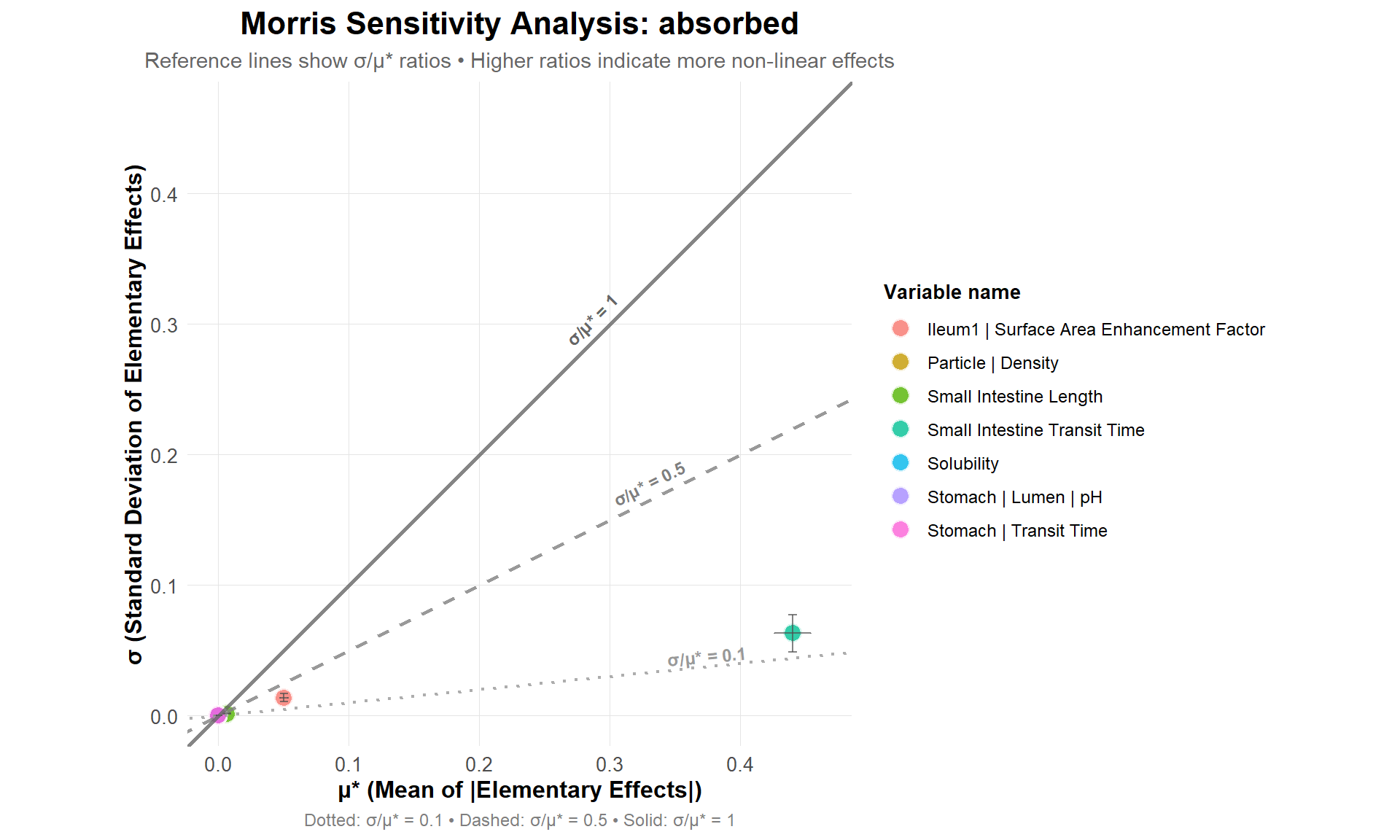

Kill GPX Service

Delete the assets created (delete_run()) or aternatively persist the changes in the project (save_project()) and then kill the GPX service after the script is executed

R

#delete_run(run_name)
#save_project()

gpx_service$kill()

CODE

[1] TRUE

References