PKPlus Example

This Jupyter notebook executes PKPlus analysis. The script utilizes the gastroPlusAPI package to communicate with the GastroPlus X 10.2 service.

The NCA output diplayed as a table.

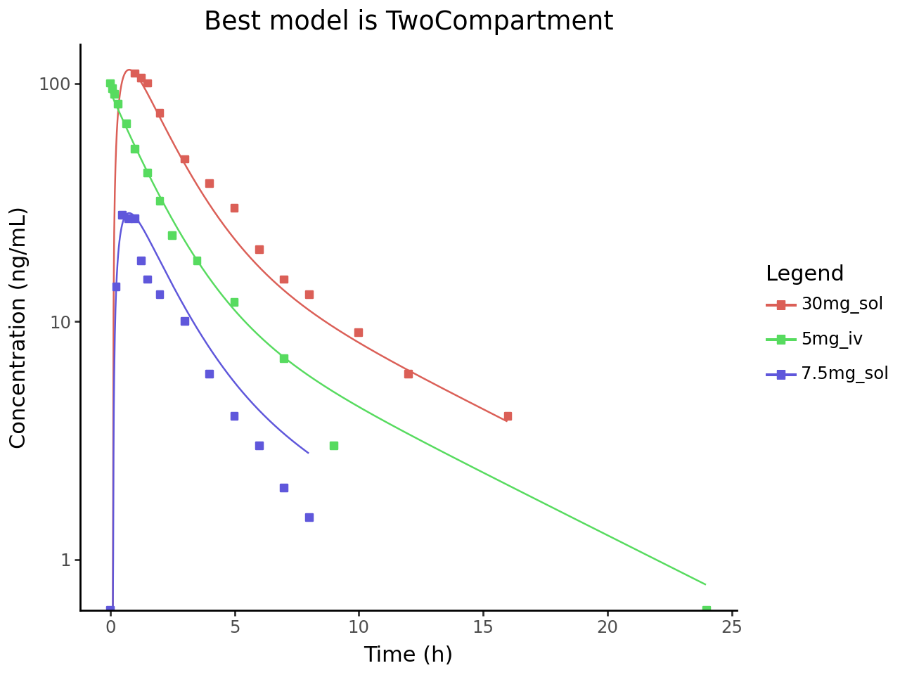
The CA output will be plotted versus the observed data.

To customize your study with this script for a different simulation / project / variables, please make changes to the “Setup Input Information” section.

Load required libraries

PY

import gastroplus_api as gp
import pandas as pd
from pprint import pprint
import os

Start the GastroPlus service

start_service() starts the GastroPlus service and stores the port the service is listening on. Alternatively, you can start the service externally and set the port variable below.

PY

try:
    gastroplus_service = gp.start_service(verbose=False)
except Exception as e:
    print(f"Error starting GastroPlus service: {e}")

CODE

GastroPlus Service configured. Listening on port: 8700

Configure and create the gastroplus client instance. The gastroplus object will used to interact with the GastroPlus Service.

If not using start_service() to start the GastroPlus service (i.e., starting externally from this script), adjust the port variable below to match the port of the GastroPlus Service instance

The port set here must match the listening port of the running GastroPlus Service.

PY

#port=8700
port = gastroplus_service.port
host = f"http://localhost:{port}"
client = gp.ApiClient(gp.Configuration(host = host))
gastroplus = gp.GpxApiWrapper(client)

Setup Input Information

Make modification to the variables in this chunk to customize your workflow.

PROJECT_DIRECTORY: Location of the GastroPlus project
PROJECT_NAME: Name of the GastroPlus project
INPUT_NAMES: Names of input for the PKPlus.
OBSERVED_DATA_GROUP_NAMES & OBSERVED_DATA_SERIES_NAMES: Observed data details to be used for plotting.
DOSE_ROUTES: Accepted values are Intravenous and Oral.
PKPLUS_RUN_NAME: Name of the PKPlus run that will include all inputs.
Bolean Parameters (True or False)
- USE_INDIVIDUAL_BW: Use individual body weight for the simulation
- FIT_F_FOR_ORAL_DOSES: Fit F for oral doses
- FIT_LAG_TIME_FOR_ORAL_DOSES: Fit lag time for oral doses
ELIMINATION_MODEL_TYPE: Accepted values are “Linear” and “NonLinear”
ANALYSES_METHODS: Choose analyses methods to be executed

PY

PROJECT_DIRECTORY = os.path.abspath("../../ProjectFiles/")
PROJECT_NAME = "Midazolam"
# Combined the above to create the full project file path
PROJECT_FILE_NAME = os.path.join(PROJECT_DIRECTORY, PROJECT_NAME + ".gpproject")
INPUT_NAMES = ["5mg_iv", "30mg_sol", "7.5mg_sol"]
OBSERVED_DATA_GROUP_NAMES = ["5 mg iv", "30 mg Solution", "7.5 mg Solution"]
OBSERVED_DATA_SERIES_NAMES = ["Plasma Conc", "Plasma Conc", "Plasma Conc"]
DOSE_ROUTES = [gp.PKPlusDoseRoute.Intravenous, gp.PKPlusDoseRoute.Oral, gp.PKPlusDoseRoute.Oral]
DOSE_MG = [5, 30, 7.5]
INFUSION_TIME_H = [0, 0, 0]
BODY_WEIGHT_KG = [70, 70, 70]

PKPLUS_RUN_NAME = "Run_for_1IV_2PO"
USE_INDIVIDUAL_BW = True
FIT_F_FOR_ORAL_DOSES = True
FIT_LAG_TIME_FOR_ORAL_DOSES = True
FRACTION_UNBOUND_PLASMA = 0
ELIMINATION_MODEL_TYPE = gp.PKPlusEliminationModel.Linear
ANALYSES_METHODS = [gp.PKPlusAnalysisMethod.NonCompartmentalAnalysis,
                    gp.PKPlusAnalysisMethod.OneCompartment,
                    gp.PKPlusAnalysisMethod.TwoCompartment,
                    gp.PKPlusAnalysisMethod.ThreeCompartment]

Configure and Execute the PKPlus Analysis Run

Based on the variables assigned in the previous code cell, the PKPlus analysis will be configured and executed

PY

gastroplus.open_project(PROJECT_FILE_NAME)

# get the observed series, we need this to link our inputs to the correct observed data
exposure_series_df = pd.json_normalize(gastroplus.experimental_data_inventory().to_dict(), record_path=['observed_series_keys'])

for index, input_name in enumerate(INPUT_NAMES):
    print(f"Adding input: {input_name}, index: {index}")
    # Get the corresponding exposure series
    exposure_series = exposure_series_df[
        (exposure_series_df["group_name"] == OBSERVED_DATA_GROUP_NAMES[index])
        & (exposure_series_df["series_name"] == OBSERVED_DATA_SERIES_NAMES[index])
    ].iloc[0]
    
    dose_amount = gp.ScalarObservable(scalar_type= gp.ScalarType.Mass,
                                      scalar_value= gp.ScalarValue( value = DOSE_MG[index], unit="mg"))
    body_weight = gp.ScalarObservable(scalar_type= gp.ScalarType.Mass, scalar_value= gp.ScalarValue( value = BODY_WEIGHT_KG[index], unit="kg"))
    infusion_time = gp.ScalarObservable(scalar_type= gp.ScalarType.Time, scalar_value= gp.ScalarValue( value = INFUSION_TIME_H[index], unit="h"))
    series_key = gp.SeriesKey(group_type = exposure_series["group_type"],
                              group_name= exposure_series["group_name"],
                              series_type= exposure_series["series_type"],
                              series_name= exposure_series["series_name"])
    pk_plus_input = gp.PkPlusAddInputBody(
        pkplus_input_name=input_name,
        dose_route = DOSE_ROUTES[index],
        dose_amount = dose_amount,
        body_weight = body_weight,
        infusion_time = infusion_time,
        exposure_series_key =series_key
    )
    gastroplus.add_pkplus_input(pk_plus_input)


# check that all inputs were added successfully, this statement will output nothing if all were successful
assert len(gastroplus.pkplus_inputs().pkplus_inputs) == len(INPUT_NAMES), "Not all inputs were added successfully"

# Add the PKPlus Run
gastroplus.add_pkplus_run(pkplus_run_name = PKPLUS_RUN_NAME, input_names = INPUT_NAMES)

# Configure the Run
ConfigurePkplusRunRequest = gp.ConfigurePkplusRunRequest(
    pkplus_run_name = PKPLUS_RUN_NAME,
    model_settings = gp.PkPlusModelSettings(
                    use_individual_body_weights = USE_INDIVIDUAL_BW,
                    fit_bioavailability = FIT_F_FOR_ORAL_DOSES,
                    fit_time_lag = FIT_LAG_TIME_FOR_ORAL_DOSES,
                    fraction_unbound_plasma = FRACTION_UNBOUND_PLASMA,
                    kinetics_type = ELIMINATION_MODEL_TYPE,
                    model_types = ANALYSES_METHODS
    )
)

gastroplus.configure_pkplus_run(configure_pkplus_run_request = ConfigurePkplusRunRequest)

gastroplus.execute_pk_plus_run(PKPLUS_RUN_NAME)

CODE

Adding input: 5mg_iv, index: 0
Adding input: 30mg_sol, index: 1
Adding input: 7.5mg_sol, index: 2

PY

pkplus_output = gastroplus.pkplus_run_output(PKPLUS_RUN_NAME).pkplus_run_output

Process NCA outputs

Get each NCA output and display it as a table. Note, while the table does not render well in this online documentation, it will render properly is VSCode or when rendered to html.

PY

nca_output = pkplus_output.to_dict()["non_compartmental_analysis_output"]
nca_df = pd.json_normalize([{"input_name": n[0], "output": n[1]} for n in nca_output])
nca_df.rename(columns = lambda x: x if x == "input_name" else ".".join(x.split(".")[1:]), inplace=True)
nca_df

	input_name	auc_first_moment_last.value	auc_first_moment_last.unit	auc_infinity.value	auc_infinity.unit	auc_last.value	auc_last.unit	body_mass.value	body_mass.unit	clearance.value	...	mean_residence_time.value	mean_residence_time.unit	terminal_elimination_rate.value	terminal_elimination_rate.unit	terminal_half_life.value	terminal_half_life.unit	volume_distribution.value	volume_distribution.unit	volume_distribution_normalized.value	volume_distribution_normalized.unit
0	30mg_sol	0.002220	(mg/mL)hh	0.000430	(mg/mL)*h	0.000403	(mg/mL)*h	70.0	kg	69815.5	...	5.16526	h	0.151206	1/h	4.58413	h	360615.20953	mL	0.005152	mL/kg
1	5mg_iv	0.000578	(mg/mL)hh	0.000213	(mg/mL)*h	0.000203	(mg/mL)*h	70.0	kg	23509.1	...	2.71539	h	0.315582	1/h	2.19641	h	63836.30000	mL	0.000912	mL/kg
2	7.5mg_sol	0.000205	(mg/mL)hh	0.000074	(mg/mL)*h	0.000070	(mg/mL)*h	70.0	kg	101797.0	...	2.78384	h	0.370244	1/h	1.87214	h	283386.56048	mL	0.004048	mL/kg

Process Compartmental outputs

Get best fitted compartmental analysis output and plot it versus observed data

PY

compartmental_output = pkplus_output.to_dict()["compartmental_analysis_output"]

cax = [{"model": c[0], "output": c[1]} for c in compartmental_output["model_outputs"]]
cax_df = pd.json_normalize(
    cax,
    record_path=["output", "predicted_concentration_series", "series"],
    meta=[
        ["output", "predicted_concentration_series", "input"],
        ["output", "predicted_concentration_series", "independent_unit"],
        ["output", "predicted_concentration_series", "dependent_unit"],
        ["model"]
    ],
)

# simplify column names
cax_df = cax_df.rename(columns={
    "output.predicted_concentration_series.input": "Legend",
    "output.predicted_concentration_series.independent_unit": "independent_unit",
    "output.predicted_concentration_series.dependent_unit": "dependent_unit"
})

# create dataframe for observed data
observed_df = pd.json_normalize(
    compartmental_output,
    record_path=["observed_concentration_series", "series"],
    meta=[
        ["observed_concentration_series", "input"],
        ["observed_concentration_series", "independent_unit"],
        ["observed_concentration_series", "dependent_unit"]
    ],
)

# simplify column names
observed_df = observed_df.rename(columns={
    "observed_concentration_series.input": "Legend",
    "observed_concentration_series.independent_unit": "independent_unit",
    "observed_concentration_series.dependent_unit": "dependent_unit"
})

# We'll only plot the results for best model, so filter rows by the 'best_model'
best_model = compartmental_output["best_model"]
cax_df = cax_df[cax_df["model"] == best_model]

Plot the best_model results compared to the observed data

PY

from plotnine import ggplot, aes, geom_line, geom_point, labs, theme_classic, scale_y_log10

plot = (
    ggplot()
    + geom_line(cax_df, aes(x="independent", y="dependent", color="Legend"))
    + geom_point(
        observed_df, aes(x="independent", y="dependent", color="Legend"), shape="s"
    )
    + labs(
        x=f"Time ({cax_df['independent_unit'].iloc[0]})",
        y=f"Concentration ({cax_df['dependent_unit'].iloc[0]})",
        title=f"Best model is {best_model}",
    )
    + theme_classic()
)
plot.show()

# Also plot with log scale
log_plot =  plot + scale_y_log10()
log_plot.show()

CODE

c:\Users\mchinander\Python\gastro-env\Lib\site-packages\pandas\core\arraylike.py:399: RuntimeWarning: divide by zero encountered in log10