Sequential and Cross PSA Run Mode

This RMarkdown file creates and executes a Sequential or Cross PSA run. The script utilizes the gastroPlusAPI package to communicate with the GastroPlus X 10.2 service.

The output from the PSA run is then used to create a 3D plot between two input variables and one output variable and a correlation plot between the input variables and the pharmacokinetic output variables.

To customize your study with this script for a different simulation / project / variables, please make changes to the “Set Input Information” section.

Configure required packages

Load other necessary packages required to execute the script
Load gastroPlusAPI package
Load gastroPlusRModuLens package

R

library(tidyverse)
library(gastroPlusAPI)
library(gastroPlusRModuLens)

Set working directory

Set working directory as the current source editor context

R

if (rstudioapi::isAvailable()){
  current_working_directory <- dirname(rstudioapi::getSourceEditorContext()$path)
  setwd(current_working_directory)
}

Start GPX Service

R

gpx_service <- start_service(verbose=FALSE)

CODE

✔ Configured the GastroPlus Service

R

gpx_service$is_alive()

CODE

[1] TRUE

Setup Input Information

Make modification to the variables in this chunk to customize your analysis.

project_path = Location of the project where PSA run will be created

simulation_name = Name of the simulation for the PSA run

psa_analysis_mode = PSA Analysis mode (Sequential / Cross)

run_name = Name of the PSA run that will be created

input_variables_tibble = Tibble containing the variable information required to setup the PSA run.

The specified user-defined variable values will be used in each simulation of the PSA run.

R

project_path = "../../ProjectFiles/GPX Library.gpproject"
simulation_name = "Atenolol 100mg PO tablet"
psa_analysis_mode = ParameterSensitivityAnalysisMode$Sequential
run_name = "sequential_psa"

input_variables_tibble <- tibble(variable_name = c("Strength", "Solubility"),
                                 spacing = c("Logarithmic", "Uniform"),
                                 lower_bound = c(50, 10000),
                                 upper_bound = c(500, 50000),
                                 variable_unit = c("milligram", "gram/meters cubed"),
                                 number_of_tests = c(10,5))

#Variables for 3d plot - choose from any input variable for PSA and summary output variables
variables_x_y_z_3d_plot = c(x= "Strength", y="Solubility", z="cmax")

Configure and Execute the PSA Run

Based on the variables mentioned in the previous code chunk, the PSA run will be configured and executed

R

#Load the project
open_project(project_path)

#Create new PSA run
create_run(run_name, RunType$ParameterSensitivityAnalysis)

add_simulations_to_run(run_name, c(simulation_name))
variable_information <- get_variable_information(run_name, 
                                                 simulation_name, 
                                                 input_variables_tibble$variable_name)
#Setup PSA Parameters List
psa_parameter_list <- vector(mode="list",length=nrow(input_variables_tibble))
count = 1

for(var in input_variables_tibble$variable_name){
  var_info <- variable_information %>% filter(input_variable_name == var) 
  
  input_info <- input_variables_tibble %>% filter(variable_name == var) 
  
  psa_parameter_list[[count]] <- PSAParameter$new(
    variable_name = var,
    baseline_value = var_info$variable_value$value,
    lower_bound = input_info$lower_bound,
    upper_bound = input_info$upper_bound,
    unit = input_info$variable_unit,
    scalar_type = var_info$scalar_type,
    number_of_tests = input_info$number_of_tests,
    spacing = input_info$spacing
  )
  
  count = count + 1
}

#Setup PSA Setting
psa_setting <- PSASetting$new(
    analysis_mode = psa_analysis_mode,
    simulate_baseline = FALSE,
    update_Kp = FALSE)

#Create PSA Configuration object
PSA_configuration <- PSAConfiguration$new(PSA_Setting = psa_setting,
                                          PSA_Parameters = psa_parameter_list)

#Create Run Configuration object
run_configuration <- RunConfiguration$new(PSA_Configuration = PSA_configuration)

#Configure the run in GPX
configure_run(run_name, run_configuration, use_full_variable_name = FALSE)

#Execute Run
execute_run(run_name)

Process run output

Get summary output and iteration records from the run just executed and create a tibble that can be used for visualization of results.

R

psa_data <- get_summary_output_tidy(run_name = run_name)

glimpse(psa_data)

CODE

Rows: 150
Columns: 13
$ compound                        <chr> "Atenolol", "Atenolol", "Atenolol", "A…
$ run_simulation_iteration_key    <chr> "sequential_psa - Atenolol 100mg PO ta…
$ simulation_iteration_key_name   <chr> "Atenolol 100mg PO tablet | Dose: 50 m…
$ simulation_iteration_key_name_2 <chr> "Atenolol 100mg PO tablet | Dose: 50 m…
$ iteration                       <int> 0, 0, 0, 0, 0, 0, 0, 0, 0, 0, 1, 1, 1,…
$ name                            <chr> "absorbed", "bioavailable", "clearance…
$ value                           <dbl> 0.4105343, 0.3991967, 27.6856569, 165.…
$ unit                            <chr> NA, NA, "L/h", "ng/mL", "(ng/mL)*h", "…
$ label                           <chr> "Absorbed", "Bioavailable", "Clearance…
$ Solubility                      <dbl> 27000, 27000, 27000, 27000, 27000, 270…
$ Strength                        <dbl> 0.05000000, 0.05000000, 0.05000000, 0.…
$ Solubility_unit                 <chr> "g/m³", "g/m³", "g/m³", "g/m³", "g/m³"…
$ Strength_unit                   <chr> "g", "g", "g", "g", "g", "g", "g", "g"…

R

#Output parameters from the PSA
psa_data %>% 
  count(name, unit, label)

CODE

# A tibble: 10 × 4
   name              unit      label                                n
   <chr>             <chr>     <chr>                            <int>
 1 absorbed          <NA>      "Absorbed"                          15
 2 bioavailable      <NA>      "Bioavailable"                      15
 3 clearance         L/h       "Clearance (L/h)"                   15
 4 cmax              ng/mL     "Cmax (ng/mL)"                      15
 5 infinite_exposure (ng/mL)*h "Infinite Exposure\n((ng/mL)*h)"    15
 6 liver_cmax        ng/mL     "Liver Cmax (ng/mL)"                15
 7 portal_vein       <NA>      "Portal Vein"                       15
 8 tmax              h         "Tmax (h)"                          15
 9 total_dose        mg        "Total Dose (mg)"                   15
10 total_exposure    (ng/mL)*h "Total Exposure\n((ng/mL)*h)"       15

Plot results in 3D plot

Derive x, y, and z data for the 3D plot from the psa_data tibble created in the previous step.

R

x_unit <- unique(psa_data[[paste0(variables_x_y_z_3d_plot[["x"]], "_unit")]])
y_unit <- unique(psa_data[[paste0(variables_x_y_z_3d_plot[["y"]], "_unit")]])

psa_data_subset <- psa_data %>% 
  filter(name == variables_x_y_z_3d_plot[["z"]]) %>% 
  rename(!!variables_x_y_z_3d_plot[["z"]] := value)

z_title <- unique(psa_data_subset$label)

# 3D surface plot for Cross PSA or 3D scatter plot for other PSA
if (psa_analysis_mode == ParameterSensitivityAnalysisMode$Cross) {
  fig <- plot_3d_surface(
    psa_data_subset,
    x = variables_x_y_z_3d_plot[["x"]],
    y = variables_x_y_z_3d_plot[["y"]],
    z = variables_x_y_z_3d_plot[["z"]]
  )
} else {
  fig <- plotly::plot_ly(
    x = psa_data_subset[[variables_x_y_z_3d_plot[["x"]]]],
    y = psa_data_subset[[variables_x_y_z_3d_plot[["y"]]]],
    z = psa_data_subset[[variables_x_y_z_3d_plot[["z"]]]],
    type = "scatter3d",
    mode = "markers"
  ) %>%
  plotly::layout(
    scene = list(
      xaxis = list(title = paste0(variables_x_y_z_3d_plot[["x"]], " (", x_unit, ")")),
      yaxis = list(title = paste0(variables_x_y_z_3d_plot[["y"]], " (", y_unit, ")")),
      zaxis = list(title = z_title)
    )
  )
}

This is a static image of the plot, in RStudio and html, one can rotate, zoom, pan, etc.

R

# Within RStudio and rendering to html, the following statement shows the interactive plot
# fig
# create a png static snapshot of the plot and display the resulting png
static_plot_image <- "psa_cross_3D_plot.png"
plotly::save_image(fig, static_plot_image)
knitr::include_graphics(static_plot_image)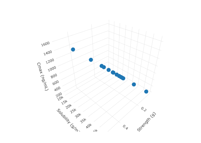

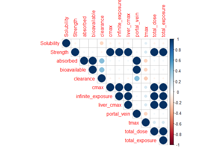
Correlation plot

R

cor_matrix <- psa_data %>%
  select(simulation_iteration_key_name, name, where(is.numeric)) %>% 
  select(-any_of(c("iteration"))) %>%
  pivot_wider(
    names_from = name,
    values_from = value
  ) %>% 
  column_to_rownames("simulation_iteration_key_name") %>% 
  as.matrix() %>% 
  cor(use = "complete.obs")

corrplot::corrplot(
  corr = cor_matrix, 
  type = "upper"
)

R

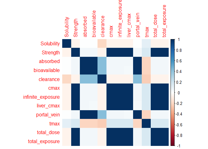
corrplot::corrplot(
  corr = cor_matrix, 
  method = "color"
)

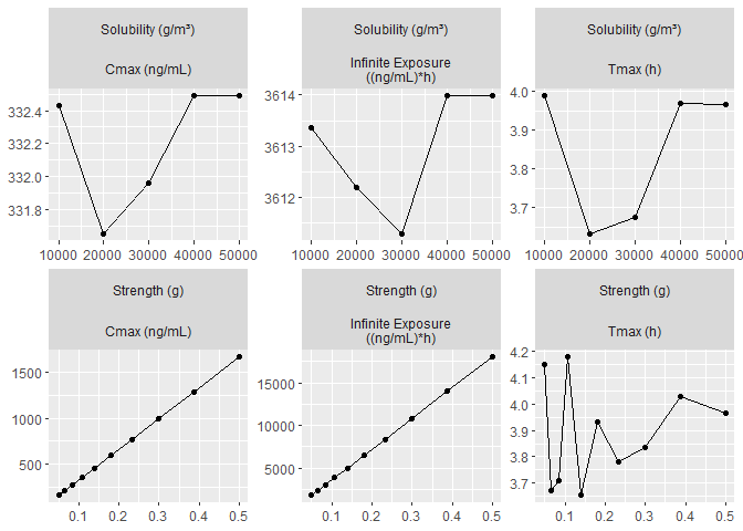
Spider plot

R

baseline_values <- psa_parameter_list %>% 
  map_dbl(~ .x$baseline_value) %>% 
  set_names(map_chr(psa_parameter_list, ~ .x$variable_name))

baseline_values

CODE

  Strength Solubility 
       100      27000

R

# amount to multiply original baseline values by to convert to output units.
unit_adjust <- psa_parameter_list %>% 
  map_dbl(function(.x) {
    input_lower_bound <- .x$lower_bound
    output_lower_bound <- min(psa_data[[.x$variable_name]])
    output_lower_bound / input_lower_bound
  }) %>% 
  set_names(map_chr(psa_parameter_list, ~ .x$variable_name))

unit_adjust

CODE

  Strength Solubility 
     0.001      1.000

R

baseline_values_adj <- baseline_values * unit_adjust[names(baseline_values)]

baseline_values_adj

CODE

  Strength Solubility 
       0.1    27000.0

R

# obtain the closest value to the baseline values.
baseline_values_closest <- baseline_values_adj %>% 
  imap_dbl(function(.x, .idx) {
    values <- psa_data[[.idx]]
    values[which.min(abs(values - .x))]
  }) %>% 
  set_names(map_chr(psa_parameter_list, ~ .x$variable_name))

baseline_values_closest

CODE

  Strength Solubility 
       0.1    27000.0

R

# Use the `spider_slice()` function to subset PSA data to suitable format for a
# spider plot.
# 
# For a sequential PSA, no subset is expected, but the additional variables
# generated by this function are expected for the spider plot.
psa_spider_data <- psa_data %>% 
  spider_slice(
    baseline_values_closest
  )

psa_spider_data %>% 
  count(parameter_name, across(any_of(names(baseline_values))))

CODE

# A tibble: 15 × 4
   parameter_name Strength Solubility     n
   <chr>             <dbl>      <dbl> <int>
 1 Solubility       0.1         10000    10
 2 Solubility       0.1         20000    10
 3 Solubility       0.1         30000    10
 4 Solubility       0.1         40000    10
 5 Solubility       0.1         50000    10
 6 Strength         0.05        27000    10
 7 Strength         0.0646      27000    10
 8 Strength         0.0834      27000    10
 9 Strength         0.108       27000    10
10 Strength         0.139       27000    10
11 Strength         0.180       27000    10
12 Strength         0.232       27000    10
13 Strength         0.300       27000    10
14 Strength         0.387       27000    10
15 Strength         0.5         27000    10

R

# Subset to select parameters.
psa_spider_data_subset <- psa_spider_data %>% 
  filter(name %in% c("cmax", "infinite_exposure", "tmax"))

plot_spider_plot(
  psa_spider_data_subset
)

Delete assets and Kill GPX Service

Delete the assets created and then kill the GPX service after the script is executed

R

delete_run(run_name)
save_project()

gpx_service$kill()

CODE

[1] TRUE