GPX™ Run Modes Tutorial: Virtual Bioequivalence

In this tutorial we will run a VBE between two Valproate formulations that have different in vitro release profiles (named ER-slow and ER-slightly slow).

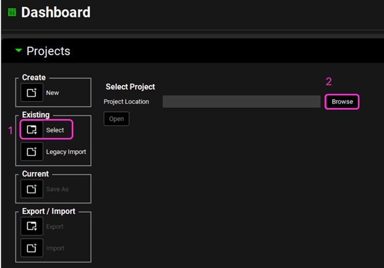
Open GPX™ and, in the Dashboard view, click on the icon next to Select to open an Existing project.
Click Browse and navigate to the C:\Users\<user>\AppData\Local\Simulations Plus, Inc\GastroPlus\10.2\Tutorials\Valproate-VBE and select the project file Valproate-VBE.gpproject by clicking on it and clicking Open.

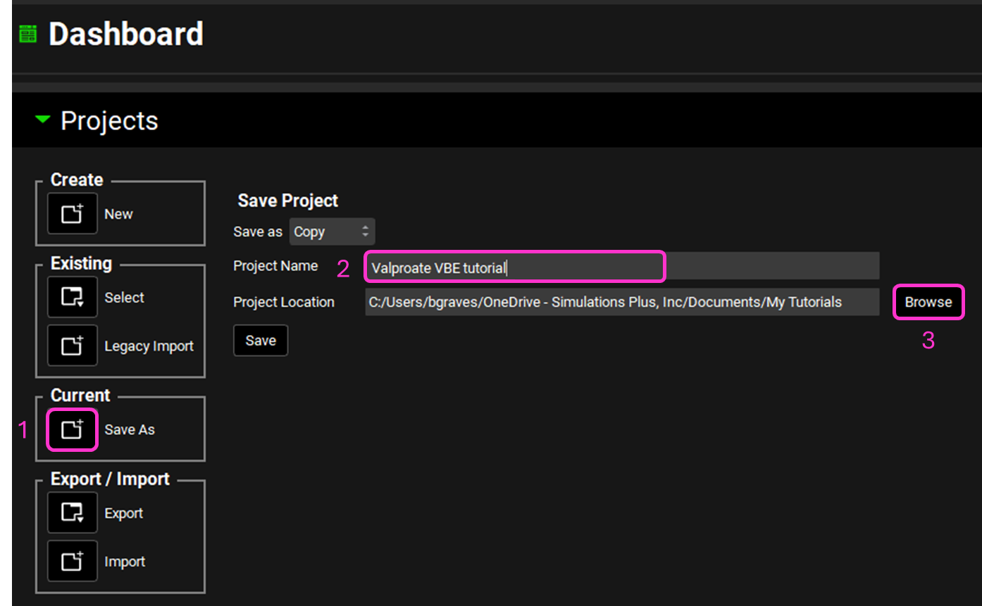
Now we will save a copy of the project to keep the original project unaltered. In the Dashboard view, click on the icon next to Save As under the Current frame. From the Save as drop-down, select Copy. Type “Valproate VBE tutorial” as the Project name and click Browse to navigate to/add a folder to Save the project in. Click Save - you will see an information message in the Messages Center indicating that the project has been successfully copied. This message will disappear once you click 'Yes' on the pop-up window that also appears.

Move through the views on the navigation pane from Observed Data to Simulations, observing the information that has been entered in this project.
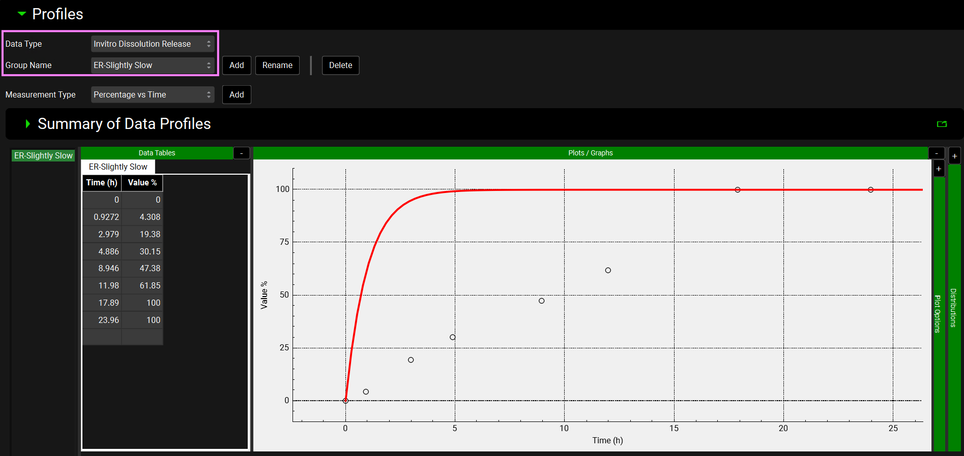
Navigate to the Observed Data view and select “In Vitro Dissolution Release” from the Data Type drop-down in the Profiles panel.
Select “ER-Slightly Slow” from the Group Name drop-down. The in vitro dissolution data for the ER-Slightly Slow formulation is shown in the graph. You may want to collapse the Summary of Data Profiles panel if open by double-clicking on the panel header bar or clicking on the green arrow.

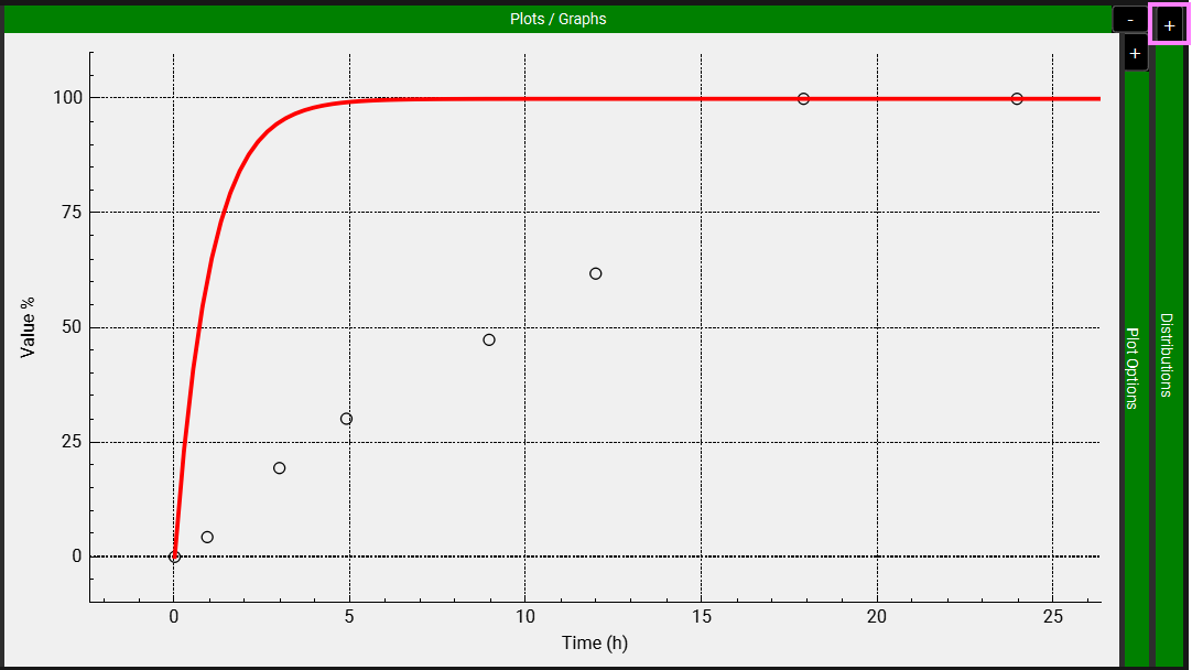
Expand the Distributions panel by clicking on the “+” at the top of the bar to access the Weibull fitting section.

Toggle Enable Distributions on if not already selected. Under Select Data, click on “ER-Slightly Slow”. In the Weibull section, leave 1 for both Number of Phases and Maximum released fraction. Make sure that the Time Lag, Maximum release fraction, Time Scale (h) and Shape toggles are on. At the bottom of the Weibull section, click on Initial Estimates and then click on Fit.

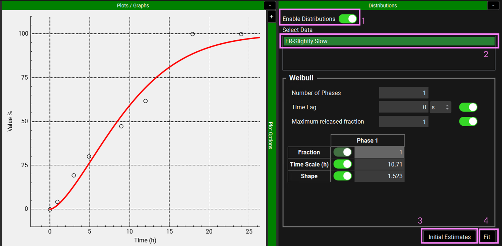
NB – numbers reflect the order of the steps in the screenshot, rather than corresponding to the steps in the tutorial.

Repeat steps 5-8 for the “ER-Slow” dissolution data.
Save the project and click on OK (or press enter).
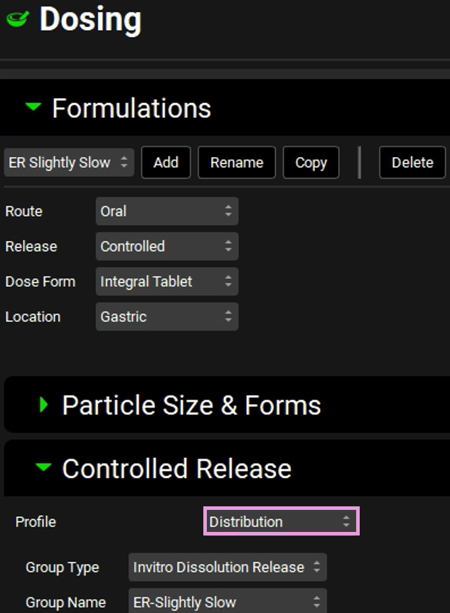
Navigate to the Dosing view and expand the Formulations panel.
Select “ER Slightly Slow” from the drop-down and expand the Controlled Release sub-panel.

Since the Release is selected as “Controlled”, the Controlled Release sub-panel is available.

From the Profile drop-down you can define the release as Tabulated data or Distribution profile (via Weibull function). Since we will be running a VBE between Slow and Slightly Slow formulations, the Weibull parameters need to be included as variables in the population simulation under the VBE Run mode. For the Weibull parameters to be shown in the VBE run mode, the Profile in the Controlled Release sub-panel must be defined as Distribution.
Select Distribution from the Profile drop-down.

Select the “ER Slow” formulation in the Formulations panel. The Controlled Release sub-panel remains open and will reflect the selections for ER Slow. Select Distribution from the Profile drop-down.

Make sure that the ER-Slightly Slow Group Name is selected for the ER Slightly Slow formulation, and ER-Slow for the ER Slow formulation.

Navigate to the Runs view and select the “Simulations” run under Run Name. The 500mg-Slow and 500mg-Slightly Slow simulations are included in this run. Click Start in the Run Controls panel.
See how there is a difference in the C_p-Time profiles due to the differences in release for these two formulations.

This plot has been formatted. When following the instructions, the plot will be in the default formatting, that is, both lines are blue, and the legend is not displayed.

Now we will assess if these formulations are bioequivalent.
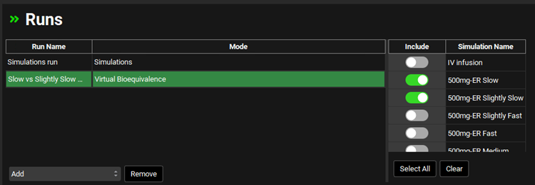
Navigate to the Runs view and click on “Virtual Bioequivalence” from the Add drop-down. The Enter Run name dialog box will appear. Name your run “Slow vs Slightly Slow VBE”. Click OK.
Move to the right-hand side and click on the Include Toggle in front of “500mg-ER Slow” and “500mg-ER Slightly Slow”.

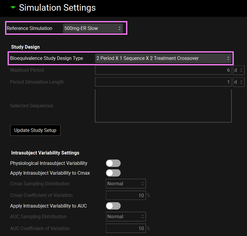
The Simulation Settings panel will be enabled. Select “500mg-ER Slow” as the Reference Simulation from the drop-down.

In this tutorial we will run a 2 Period, 1 Sequence and 2 Treatment Crossover VBE. Select this option from the Bioequivalence Study Design Type. We will not assign any intrasubject variability, so leave the Intrasubject Variability Settings untoggled.

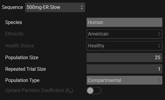
Scroll down to the Sequence drop-down and select “500mg-ER Slow” if not already selected. We will use the following population characteristics for this VBE: Species: Human, Ethnicity: American, Health Status: Healthy, Population Size: 25, Repeated Trial Size:1 and Population Type: Compartmental.

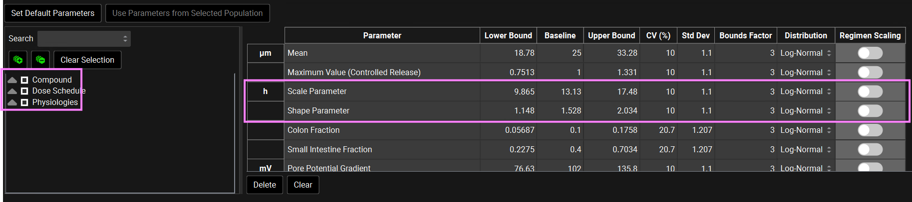
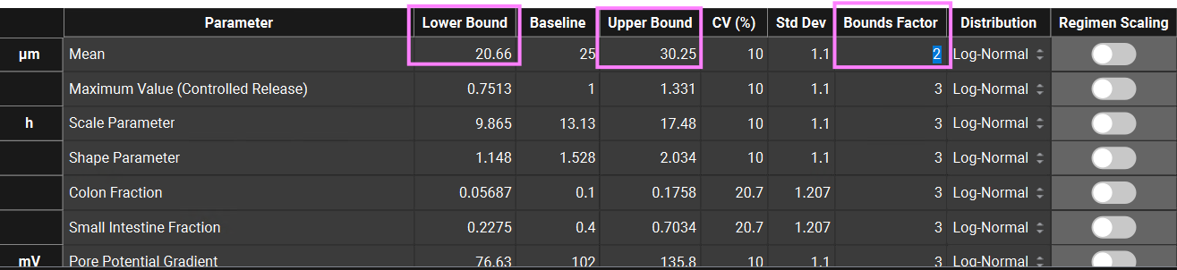
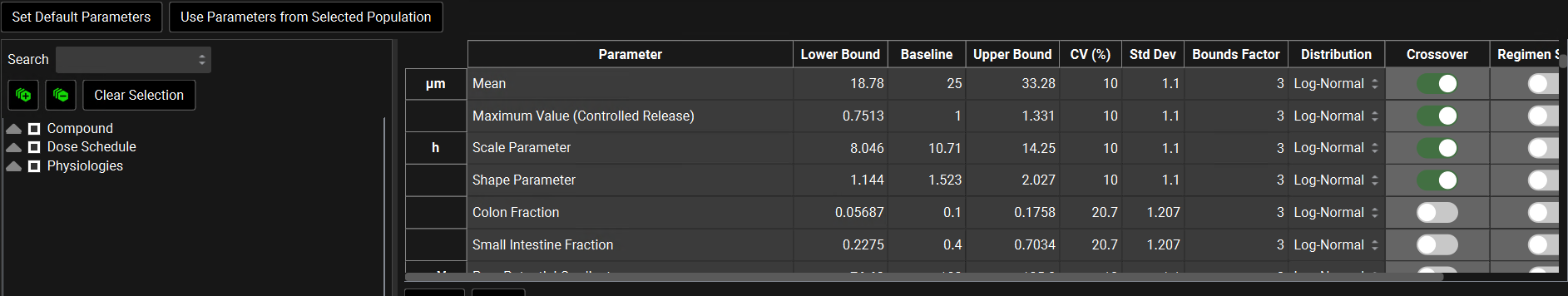
Scroll down to the parameters table wherein the default parameters are selected. Default coefficients of variation and distribution types are also shown. You can use the parameters list on the left-hand side to change the selection of variables by expanding the list or typing the variable name in the Search box. Note that the Weibull Scale and Shape parameters have been automatically selected. The Baseline values reflect the fitted values in the Observed Data view.

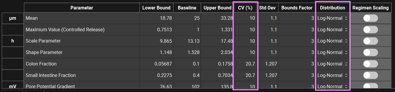
You can change each CV (%) if you wish by directly editing it in the table. Select the type of distribution you want for each variable (Normal, Log-Normal, or Uniform), and enter the CV for that distribution (for Log-Normal, enter the CV of the log of the variable).

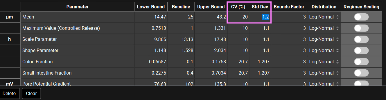
In GPX™ you also have the flexibility of adjusting the standard deviation (Std Dev). For example, you could set the Std Dev to 1.2 to get a CV% of 20% for a Log-Normal distribution.

The Bounds Factor defines the constraints for the lower and upper bounds. For example, if the Bounds Factor is 3 (default), that means the lower and upper bound are 3 standard deviations. If you wish to constrain everything to 2 standard deviations, you can set the Bounds Factor to 2 and so on.

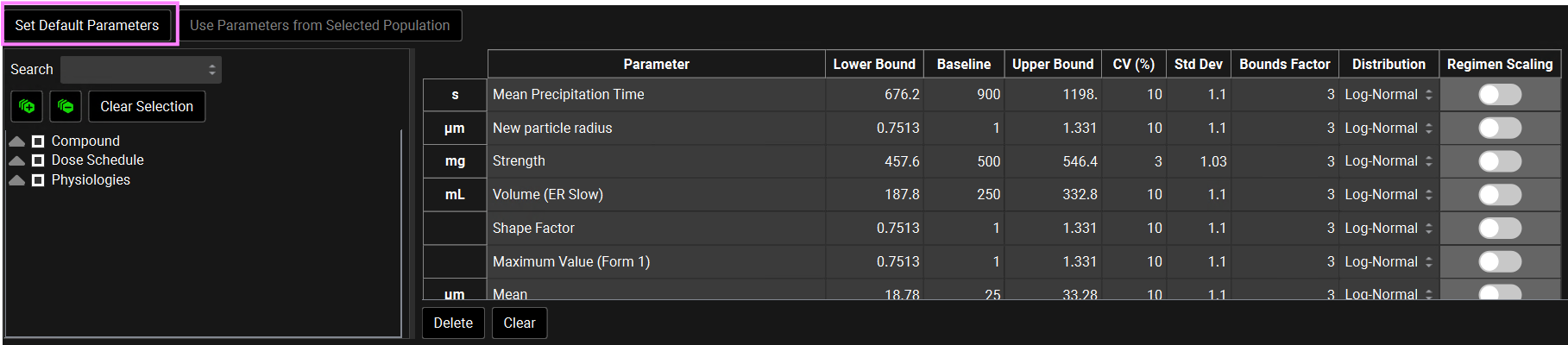
If you have made changes but would like to go back to the default values, you can click on the Set Default Parameters button to restore the selection and values to the default values. In this tutorial we will run a VBE with all default parameters and CVs. If you have changed any parameters, click on Set Default Parameters before continuing.

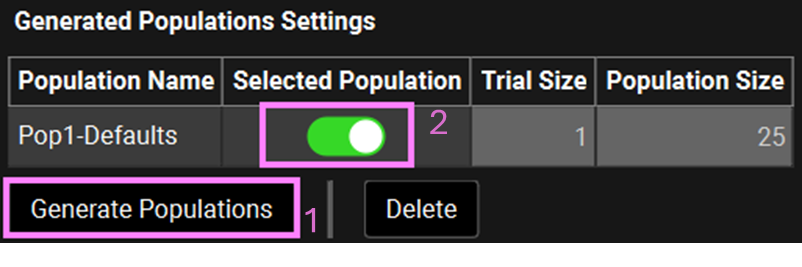
Scroll down to the Generated Populations Settings table. Click on Generate Populations and name it as Pop1-Defaults. Toggle on the Selected Population Toggle.

Using “User Defined Output Points” in the simulations included in the VBE run is a best practice to avoid differences in AUC, Cmax and Tmax between runs using the same population. This setting is found under “Configuration” panel in “Simulations” view.

Scroll up to see that some parameters such as Population Size and Repeated Trial Size are grayed out. This is because a population is toggled in the table below. If you wish to create another population with different characteristics, untoggle the selected population in the Generated Populations Settings table.
Scroll down to the Generated Populations Settings table and select the Pop-1-Defaults. Click on Use Parameters from Selected Population so that the parameter table reflects the selected population.

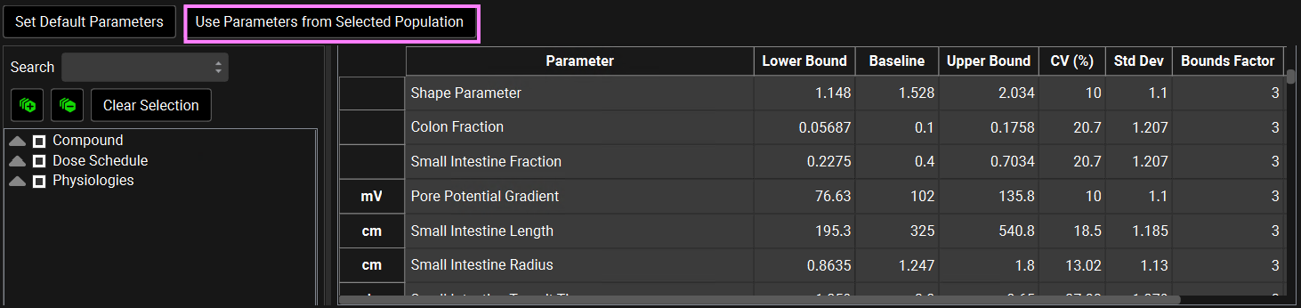
Scroll up and select the 500mg-ER Slightly Slow from the Sequence dropdown. Scroll down to the parameters table and note that the Weibull Scale and Shape parameters now reflect the fitted values in the Observed Data view for the Slightly Slow formulation.

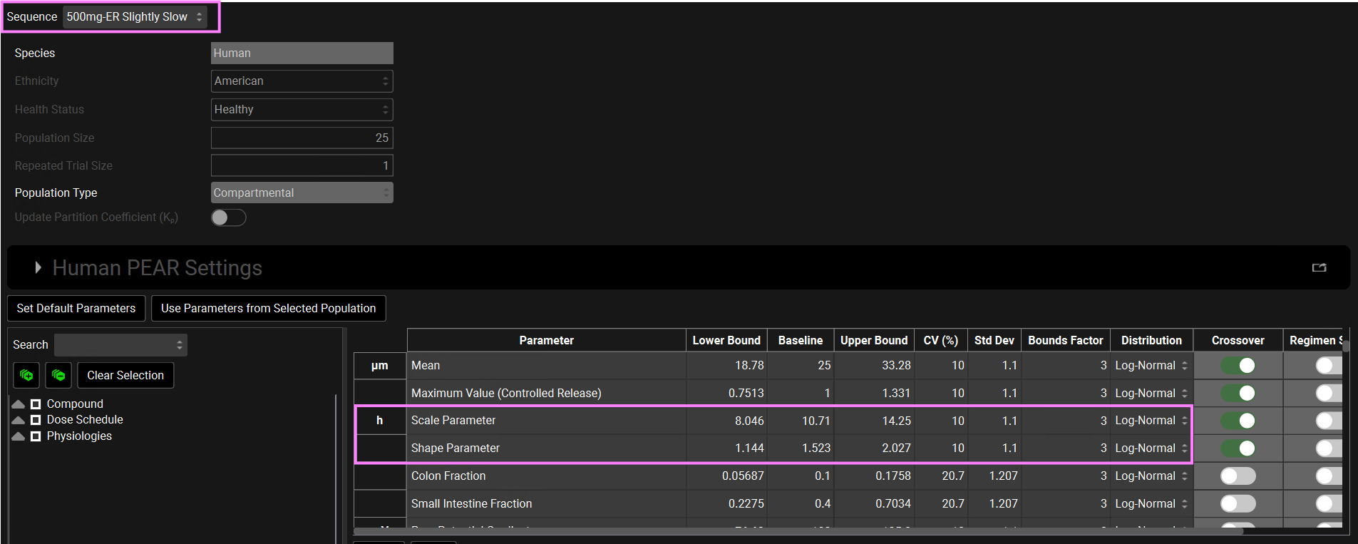
When the test simulation is selected (ER-Slightly Slow in this tutorial) a “Crossover” column appears in the parameters table. You might need to slide the bar to the right to see the Crossover column. The parameters that have the toggle on will have different sampled values between the two population simulations. The parameters that have the toggle off will be the same in the test simulation as sampled in the reference population. The Regimen Scaling toggle indicates gut physiological parameters (such as transit times, intestinal fluid volume, pH values, and bile salt concentrations for each gut section) that will be scaled in the second period when applicable.

Note: These toggles are not editable. It simply indicates how the parameters are going to be sampled.

Save the project and click on OK (or press enter).
Scroll down to the Run Controls panel and click on Start.
The Analysis view will automatically appear when the Run has completed.
The Population View mode is automatically selected for a virtual bioequivalence run and will display the mean C_p-Time curve and the 90% confidence interval for both Slightly Slow and Slow formulations.

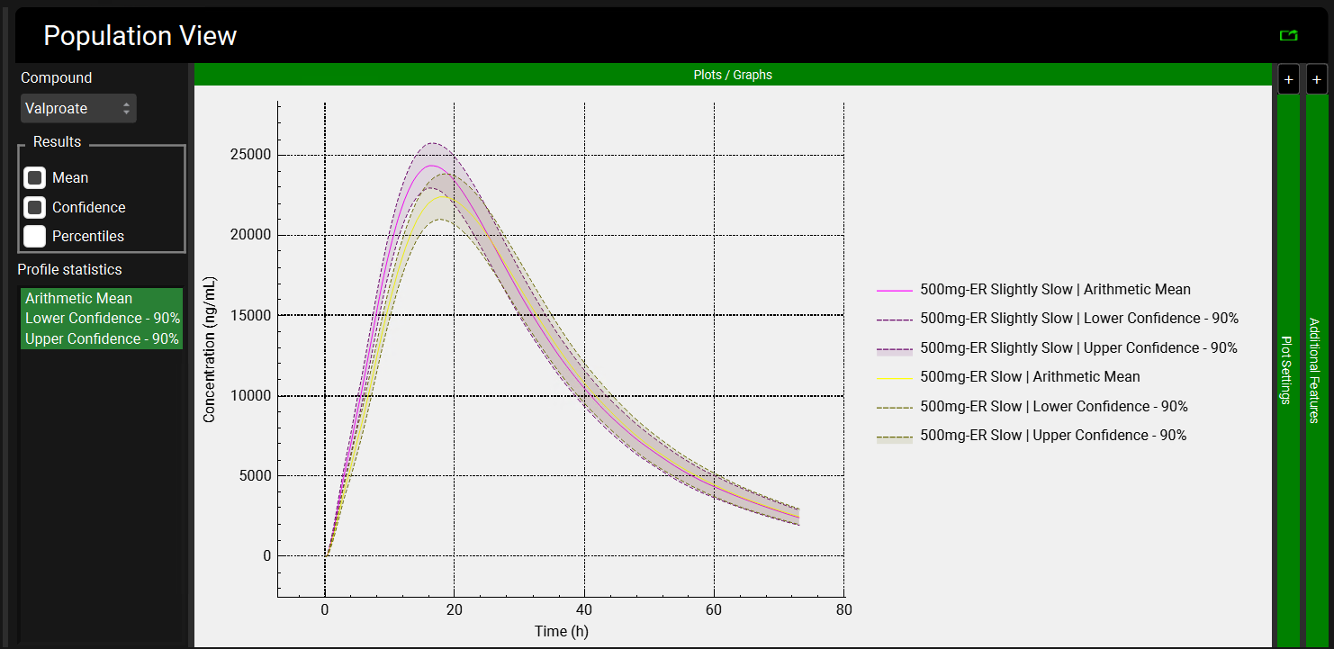
This plot has been formatted to show the legend on the right-hand side. When following the instructions, the plot will be in the default formatting, that is, the legend is not automatically displayed.

Because Population Simulator is based on random samples, your results will most likely be somewhat different than the results shown above.

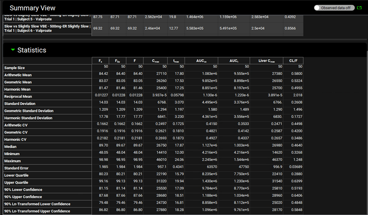
Switch the Mode to Summary View, which enables you to see the F_a, F_Dp, F, C_max, T_max, AUC, Liver C_max and CL/F for each subject in this population for each administration period.

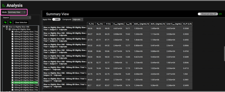
Scroll down to the Statistics panel and expand it. Note how Sample Size (first row in the Statistics table) is 50. This is the overall statistics for the two sequences of population runs (25 subjects each) in this virtual bioequivalence.

On the Run list located left of the Summary View panel, unselect the 50mg-ER Slightly Slow simulations by clicking on the box next to it.

You may have to click on the box twice to unselect everything. The first time you click, it will go from a filled square to a tick. After that, click on it again to unselect all the curves.

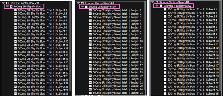
Once the selection has been cleared, the Summary and Statistics tables will reflect only the 500mg-ER Slow population simulation. Note that the Sample Size in the Statistics table now reads 25.
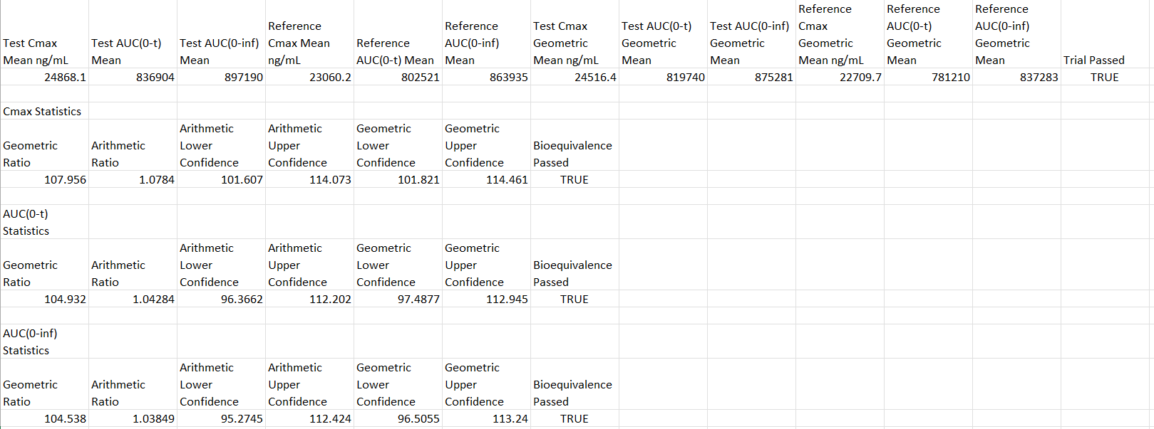
Open one of the automatically generated output files that is saved in the VBE project folder (e.g.: 500mg-ER Slightly Slow Valproate Trial 1 BE Stats.xlxs) to assess if the trial passed the 80%-125% BE criteria. (Note: the file name will also have a time and date stamp prior to the .xlsx).

The VBE results can also be plotted on the graph. In the Population View, expand the Additional Features by clicking on the “+” sign on top of the bar. Select one of the periods and and toggle on Bioequivalence Statistics.

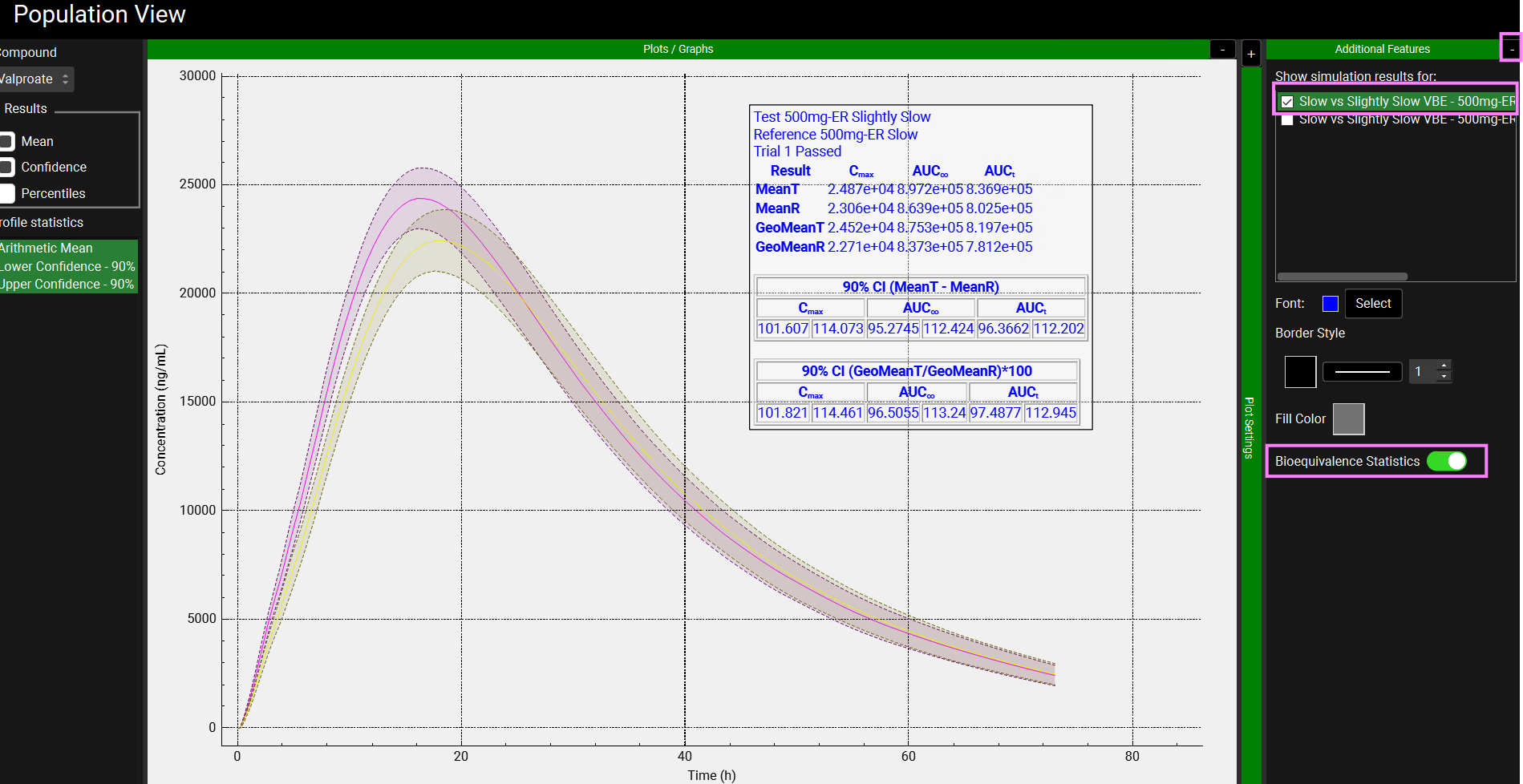
Because Population Simulator is based on random samples, your results will most likely be somewhat different than the results shown above.