Solubility and Dissolution Models

The ACAT model assumes that only drug in solution can undergo lumenal degradation, carrier-mediated influx transport, absorption into the intestinal wall via the transcellular pathway, or absorption into the portal vein via the paracellular pathway.

After drug has been absorbed, it is assumed to remain in solution in enterocytes, plasma, and all PK compartments.

Thus, both the rate at which solid drug particles dissolve and the total amount of drug that can be dissolved in any compartment at any time (the solubility) have a direct effect on the degradation, efflux, metabolism, and absorption of a drug. Some lipophilic drugs can be incorporated into bile salt micelles and achieve solubilities that are greater than in water. GastroPlus® can account for the changes in solubility due to the concentration of bile salts in each region of the small intestine and has built-in bile salt concentration data for both fed and fasted conditions for human and preclinical species. For ionizable compounds, both the total amount of material that can dissolve at any point and the rate of dissolution partially depend on the local pH. If the drug in solution transits from a compartment of high solubility to one of lower solubility, then precipitation can occur. The rate of precipitation can affect the oral plasma concentration (C_p) versus time profile.

As shown in Figure 1-1, the ACAT model differential equations define three parallel series of transit sub-compartments to accommodate unreleased drug, undissolved drug, and dissolved drug. The model can also use measurable data for predicting lumenal degradation, which is the process of degrading the dissolved drug in the dissolved sub-compartments.

Undissolved drug undergoes transit and dissolves to give dissolved drug. Dissolved drug undergoes transit, lumenal degradation, and absorption. If the concentration of the dissolved drug exceeds the local solubility within a particular compartment, then the dissolved drug can also precipitate and become undissolved.

Transit of any drug form—unreleased, undissolved, or dissolved—is allowed only to the same sub-compartment of the next compartment. For example, undissolved drug can transit only to the undissolved sub-compartment of the next compartment. Changes in form—unreleased to undissolved or dissolved, undissolved to dissolved, and dissolved to absorbed, undissolved, or degraded—are allowed to occur only within a compartment.

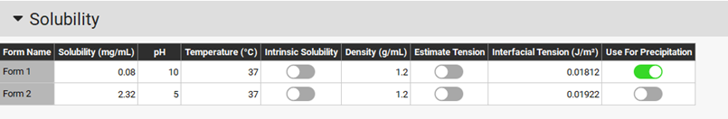
Solubility

The Dissolution process is the process that gets drug into solution. Solubility is one of the compound properties that must be used as an input for the Dissolution models and the Precipitation models, and therefore, is discussed first.

Generally, ionized molecules have greater aqueous solubility than their un-ionized forms; thus, organic acids are more soluble at higher pH values and organic bases are more soluble at lower pH values. This general principle is the basis for the calculation of the pH- dependence of solubility in GastroPlus®. Molecules with both acidic and basic functional groups can form zwitterions that have lower aqueous solubility than either the cationic form at low pH or the anionic form at high pH. GastroPlus® accepts compounds with multiple ionizable groups in its calculation of the total percent ionized. This allows the simulation to account for the dissolution profile of zwitterions or ampholytes.

To estimate the solubility of a drug at specific pHs, three variables are required:

• Solubility factor (SF) of the drug, which is the ratio of the solubility of completely ionized drug to completely unionized drug. These values are known to vary from < 10 to over 10⁶ for different compounds, with higher values for compounds with lower intrinsic solubilities. The rough rule for estimating the SF for a drug is:

SF = 20/(intrinsic solubility in mg/mL)

• All pKas for the drug.

• The solubility of the drug at any single pH.

GastroPlus® uses the following pH profiles for the human small and large intestines based on experiments performed by continuously determining the pH with time ^{1 2 3} .

Another important aspect that affects in vivo dissolution of a drug is the presence of bile salts in the small intestine. GastroPlus® includes an equation (Equation 1-5) to account for the difference between aqueous and in vivo solubility due to the presence of bile salts in the small intestine ⁴ . The calculated value is then used in the Dissolution model.

Equation 1-5: Difference between aqueous and in vivo solubility caused by the presence of bile salts

where:

Equation 1-6:    Theoretical prediction of SR based on logP

Bile salt concentrations in individual small intestine compartments in fasted and fed state were calculated based on published values for human ⁶ , rat, and dog ⁷ . Because of the lack of information for other preclinical species, the bile salt concentration profile derived for humans is currently being used for all remaining preclinical species.

Effect of surfactants on drug solubility

Bile salts or other synthetic surfactants can be used in dissolution media to increase the solubility of the drug of interest and achieve sink conditions. The affinity to surfactants depends on the drug lipophilicity and micelle surfactant type. Drugs may be able to adsorb at the surface of the micelle, form mixed micelle with the surfactant or penetrate the micelle hydrophobic core if it exists. Other factors like pH, ionic strength for ionic micelles can also alter the partitioning of the drug to the micelles since these parameters can change the nature and intensity of intermolecular force balance for the drug in the aqueous environment and the micelle. Finally, the micelle concentration may also play a role since the size, shape and type of micellar phase may change with surfactant concentration. For very low surfactant concentrations, below the critical micelle concentration (CMC), the surfactant exists as solute in the aqueous phase. With increasing surfactant concentration, the surfactant will form aggregates, micellar, tubular, or lamellar phases. These phase transitions may affect how the drug solubilizes in the micelle. Finally, for ionic surfactants which bear a specific counterion like Na+, Br-, or Cl- in Sodium docedyl sulfate (SDS),  dodecyltrimethylammoniumbromide (DTAB), or tetradecyltrimethylammonium chloride (TTAC) respectively, adding extra-counterion in the medium, typically from the buffer used to control the medium pH can affect the size and CMC of surfactants. To model the effect of surfactant on solubility and dissolution one important factor to measure is the drug affinity to the surfactant in given experimental conditions (typically those of the in vitro dissolution medium)

The affinity to surfactant: () when micelles are formed is provided in mg/mL/mM surfactant or mg/mL/percent surfactant depending on the unit of surfactant concentration in the dissolution medium. is the slope of the apparent drug concentration above the critical micelle concentration as function of the surfactant concentration.

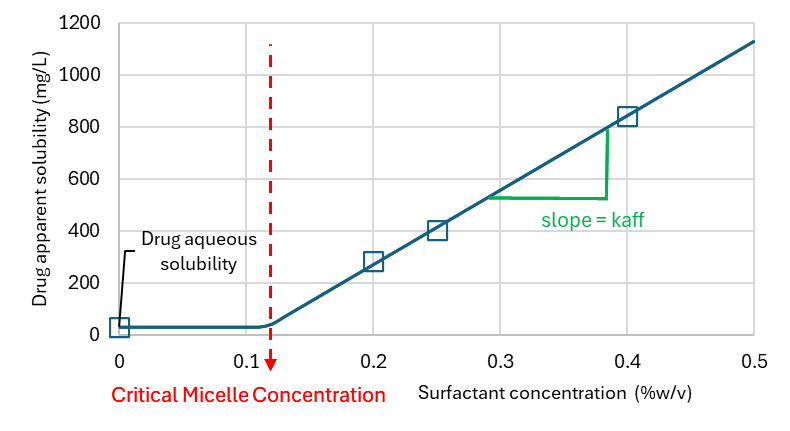
can be fitted from apparent drug solubility in the presence and absence of surfactant using the following equation, where is the apparent drug solubility, is the drug solubility in the blank medium (without surfactant), is the surfactant concentration and  is the surfactant critical micelle concentration.

Equation 1-7: Apparent Solubility of Drug in Presence of Surfactant

Note that if , then .

When micelles are formed is provided in mg/mL/mM surfactant or mg/mL/percent surfactant depending on the unit of surfactant concentration in the dissolution medium. is the slope of the apparent drug concentration above the critical micelle concentration as function of the surfactant concentration.

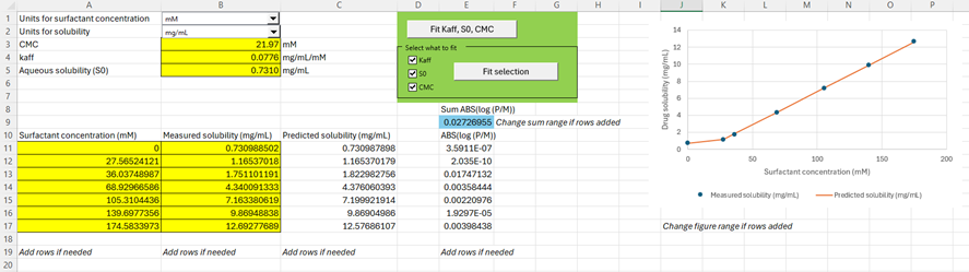
Within the Help menu in GPX™, you can access a fitting tool to calculate the parameters , , and . Download the file Kaff-fitting-tool.xlsm from here ( Kaff-fitting-tool-v1.0.xlsm). Allow the macros to run upon first opening.

Select the units for Surfactant concentration and solubility of your experiment using the drop-down menus provided. Add your solubility data as function of surfactant concentration in the range starting from A11:B11. Seven rows are provided for your data entry, and you can add more rows is needed. If you do add more rows, remember to change the sum formula of cell E9. You have two choices for fitting your parameters: Either fit all parameters to the data or select the parameters you want to fit. You can manually change the , , or aqueous solubility prior to fitting the other selected parameters. You can copy the and data in GPX™ for further utilization in dissolution rate prediction using the P-PSD approach.

Cyclodextrin formulations for increasing aqueous solubility

Cyclodextrins are cyclic oligosaccharides. They pharmaceutical adjuvants used as complexing agents to increase the aqueous solubility of active substances that are poorly soluble in water. The molecular structure of these glucose derivatives, which approximates a truncated cone, bucket, or torus, generates a hydrophilic exterior surface and a non-polar interior cavity. Cyclodextrins can interact with appropriately sized drug molecules and bind drug molecules 1:1 into their central cavities. The binding is reversible and can be described by a simple binding constant, K_{_assoc}, as shown in Equation 1-8.

Equation 1-8:  Cyclodextrin binding constant

where:

Dissolution models

In GastroPlus®, you can calculate dissolution using one of three models:

• The Johnson (default) model ⁸

Equation 1-9:    Default model equation for dissolution rate

• The Wang-Flanagan model ^{9 10}

Equation 1-10:    Wang-Flanagan model equation for dissolution rate

• The Z-Factor model ¹¹

Equation 1-11: Z-Factor model equation for dissolution rate

where:

The z factor in Equation 1-11 represents the term shown in Equation 1-12 and is obtained by fitting the equation to in vitro dissolution data, where D_wis the diffusivity of the drug in water. The remainder of the variables are defined in the table above.

Equation 1-12: Term represented by the z factor

Five variables can be taken into consideration in a Dissolution model:

• The diffusion layer thickness. See Diffusion layer thickness.

• The effective diffusion coefficient. See Effective diffusion coefficient.

• The particle radius. See Particle radius.

• The effect of particle size on solubility. See Effect of particle size on solubility.

• The aqueous solubility of the drug due to its formulation. See Cyclodextrin formulations for increasing aqueous solubility.

Diffusion layer thickness

Empirical evidence suggests that diffusion layer thickness is of the order of the particle radius for particle radii up to 30 μm. The Johnson (default) model and the Wang-Flanagan model use diffusion layer thickness that is equal to the particle radius up to an upper limit of 30 μm; however, the models also include an option to use a constant diffusion layer thickness that is independent of particle size. The diffusion layer thickness is not applicable for the Z-Factor model.

Effective diffusion coefficient

The effective diffusion coefficient (D_eff) is calculated according to Equation 1-13.

Equation 1-13: Effective diffusion coefficient calculation

where:

Okazaki ¹²  has shown that the size of an aggregate, and subsequently, its diffusion coefficient, is a function of phospholipid and bile salt concentrations and is not significantly affected by saturation with the dissolved drug. The relationship between the D_agg and bile salt concentration was fitted to published data and is used within GastroPlus® to calculate D_eff in each compartment. If the option to adjust the diffusion coefficient for bile salt effect is not selected, then D_eff is assumed to be equal to D_mono.

Particle radius

Two particle size distribution options are available for calculating the particle radius:

• Monodisperse – All particles have the same size.

• Polydisperse – The formulation is a mixture of different particle sizes.

GastroPlus® has two built-in probability density functions—Log Normal and Normal—that are used for setting up initial particle size distributions. (A user-defined distribution option is also available.) These distributions are divided equally into spaced bins, and then normalized to 100% to calculate the initial mass of undissolved drug that corresponds to each bin.

• Log-Normal distribution

Equation 1-14 defines the probability density function for the Legacy Log-Normal distribution.

Equation 1-14: Probability density function for the Legacy Log-Normal distribution

where:

Equation 1-15 is the calculation for the lower radius limit and Equation 1-16 is the calculation for the upper radius limit. These values can be edited if only a fraction of the overall distribution was used in the current formulation.

Equation 1-15: Lower radius limit, Legacy Log-Normal distribution

Equation 1-16: Upper radius limit, Legacy Log-Normal distribution

• Normal distribution

Equation 1-17 defines the probability density function for the Normal distribution.

Equation 1-17: Probability density function for the Normal distribution

where:

Equation 1-18 is the calculation for the lower radius limit and Equation 1-19 is the calculation for the upper radius limit. These values can be edited if only a fraction of the overall distribution was used in the current formulation.

Equation 1-18: Lower radius limit, Normal distribution

Equation 1-19: Upper radius limit, Normal distribution

Optionally, you can decide if the dissolution process is to affect the particle radius or if the particle radius should be kept constant for the purposes of the dissolution rate calculation.

For quickly dissolving compounds, the option of keeping a constant radius can provide adequate results while increasing the simulation speed.

If the dissolution process affects the particle radius, then the particle radius is adjusted to the remaining undissolved amount as shown in Equation 1-20.

Equation 1-20: Adjusting the particle radius to the remaining undissolved amount

where:

If the particle radius decreases in response to the dissolution process, then the diffusion layer thickness decreases accordingly. In all cases when particle diameters become less than 10 nm, GastroPlus® ceases to include them in the integration.

If the particles are non-spherical, then the particles in all bins are considered to be the same shape and the same shape factor is applied to all particles and is kept constant throughout the simulation.

The drug is assumed to be dissolving evenly from the entire surface of the particles and not affecting the particle shape.

Effect of particle size on solubility

The solubility for particles of a specific radius is calculated from the Kelvin equation.

Equation 1-21: Kelvin equation

where:

If all temperatures are specified, then the solubility with no curvature at temperature T (Cs,T) is calculated from the reference solubility as shown in Equation 1-22, with the calculation of the value of K (the reference solubility) shown in Equation 1-23.

Equation 1-22: Solubility with no curvature at temperature T

Equation 1-23: Calculation of K in Equation 1-22

where:

Several published studies ^{13 14}  showed significantly higher bioavailability of poorly soluble drugs after dosing formulations consisting of nano-sized API particles when compared to formulations with particles in the micron range. The increase was much higher than expected based on a faster dissolution due solely to an increased surface area and/or to a solubility increase described by the Kelvin equation. One hypothesis is that this effect could be caused by a local '”supersaturation” when the nano-sized particles get trapped between apical microvilli. The dissolution of these trapped particles in this limited volume would result in a higher local concentration of dissolved drug, which, in turn, creates a higher apical concentration gradient and therefore increases the flux across the apical membrane.

An equation based on this “super-saturation” hypothesis has been incorporated into GastroPlus®. The equation adjusts the solubility of the compound that is used in the Dissolution model. The local supersaturation is given by the NanoFactor Effect (NFE). This effect specifies the extent by which a drug can dissolve from these nano-sized particles to concentrations that exceed the local solubility limit. The NFE for different particle sizes is calculated using an empirical equation shown in Equation 1-24.

Equation 1-24: Nanofactor Effect calculation

where:

Simulations Plus calibrated the NFE equation using the Cp versus time data for several formulations of aprepitant with particle diameters ranging from 5.5 microns to 0.12 microns. Because the equation was calibrated based on particle diameter, (2r), Simulations Plus determined the default value of NF to be 0.5.

Using the P-PSD models

If a surfactant is used in the dissolution medium, f_u the fraction of free drug in the medium is given by:

Equation 1-25: Fraction of Unbound Drug in Solution

where C_u(t) is the unbound drug concentration at all times and C(t) the total drug concentration at all times. Equilibration is assumed to be instantaneous and so f_u is anticipated to be constant. The affinity to surfactants k_aff, is experimentally determined to apparent solubility vs surfactant concentration (C_surf) in each dissolution medium (See Effect of surfactants on drug solubility).

For the P-PSD approach, the in vitro dissolution rates are fitted according to the film theory, i.e. controlled by the drug diffusion through a stagnant film layer surrounding the dissolving particle called the unstirred water layer (UWL) ¹⁵ . The Nernst-Brunner equation, which describes the variation of amount of undissolved drug dm_solid (kg) with time for a solid particle is modified to take into consideration the binding of drug to micelles and the diffusion coefficient of micelles and pure drug out of the unstirred water layer. This equation is close to the one developed by Gamsiz et al. ¹⁶ , although the treatment of fraction drug unbound and thickness in UWL differ from the approach taken by these authors ¹⁷ .

Equation 1-26: Dissolution Rate Calculation

Where A(t) (m²) is the surface area of the particle at time t, D_u and D_b the diffusion coefficient of the unbound drug and micelle-bound drug respectively (m².s^-1), h_u and h_b the UWL thickness of the unbound drug and micelle-bound drug respectively (m), C_S,u is the unbound drug solubility at the surface of the drug crystal and C_u, the unbound drug concentration in the bulk (kg.m^-3). This equation sums up the flux of drug dissolving from the crystal surface as free and micelle bound drug.

The term  and the expansion of the above equation leads to:

Equation 1-27: Dissolution Rate Expanded Equation

Where and are the micelle-bound drug concentrations at the surface and in the bulk. The hypotheses behind this equation are: 1) the flux of unbound and micelle-bound drug depend on their respective concentration differences across their UWLs and 2) the binding to the micelle in the UWL or in the bulk is immediate and sequential to the release of free drug, which reduces the amount of free drug by a factor fu.

The inclusion of hydrodynamics in the dissolution model relies on different models to calculate the thickness of the unstirred water layer (UWL). Two additional models for P-PSD are available which integrate the fluid velocity in USP2 dissolution apparatus, the P-PSD HD, and one model predicting drug and excipient sedimentation and cone formation at the bottom of the USP2 vessel, the P-PSD HDC ¹⁸ . These latter models are important to remove the potential bias coming from formulation sedimentation or to integrate the impact of fluid velocity in USP2, which would be important for large particles or large dosage forms such as eroding tablets or pellets ^{19 20} . The P-PSD HD and P-PSD HDC models are both available for download here ( P-PSD-HD.xlsx and P-PSD HDC-1_2_model.xlsx).

For the classical P-PSD approach, the assumption is that the thickness for the UWL of the unbound drug is assumed equivalent to the particle radius for small particles as long as the particle radius is below 30 µm and 30 µm for particles ≥ 30 μm ²¹ . As the dissolution proceeds, the particles shrink and this stagnant film layer will be reduced as well according to time. This approximation for the thickness of the UWL is valid for small particles. When particles will become larger or when the hydrodynamics in the model will be increased, the particles may experience different velocity profiles relative to the fluid flow which will change the thickness of the UWL. The thickness of the UWL for the micelle-bound drug is calculated based from the diffusion coefficients of the free drug and the micelle-bound drug according to the following equation ²² :

Equation 1-28: Characteristic Length Scale for Diffusion

The free drug or micelle-bound drug diffusion coefficients D (m².s^-1) are obtained from literature data or from the Stokes Einstein equation, assuming that the molecular shape is a sphere of radius r_h (m):

Equation 1-29: Stokes-Einstein Equation for Diffusion Coefficient

Where k = 1.3806504 10^-23 (J.K^-1) is the Boltzmann constant, T is the absolute temperature in kelvin, η (Pa.s) is the dynamic viscosity of the solvent and r_h (m) is the hydrodynamic radius of the diffusing solute. The hydrodynamic radius of the solute can be estimated, assuming that the molecular shape is a sphere and that the hydration of the solute is negligible, by the following equation:

Equation 1-30: Calculation of Diffusion Coefficient in Water

Where M_W is the molecular weight of the drug (g.mol^-1), N_A = 6.02214179 10²³ (mol^-1) is the Avogadro number and ρ_S is the drug true density in (kg.m^-3). The effect of temperature for dissolution is accounted for by a change in the water viscosity.

For micelles, a database of micelle size is provided in GPX™ to select baseline values for the simulation. The size of micelles is vastly different which can lead to widely different diffusion coefficients.

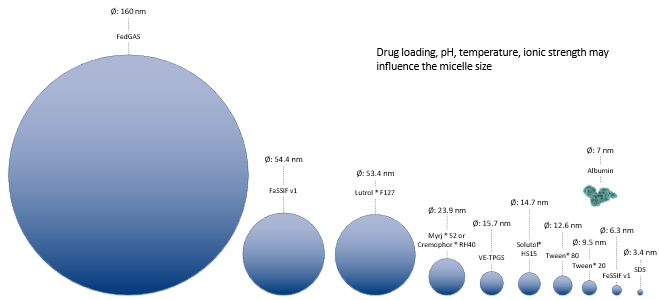
The database within GPX™ will provide starting values for micelle size. Note that since the temperature, counter-ion concentration and surfactant concentration will affect the size of micelles and also the CMC of the micelles, an additional tool is available from the help to be able to refine the size and CMC of micelles in given media. To access this tool, download the “Size and CMC calculator.xlsm” file here ( Size and CMC calculator-v1.0.xlsm).

From the welcome page, click on the button “Launch CalcSurf v1.0”.

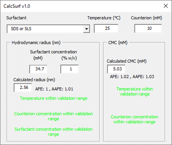
From the surfactant drop down menu, select the surfactant of interest. Indicate the temperature of the medium (°C) and counterion concentration (mM) if the surfactant is ionic. Then indicate a surfactant concentration for the calculation of micelle hydrodynamic radius. The tool will indicate whether the input parameters are within the validation range and what are the model prediction performance in terms of Average Fold Error (AFE) and Absolute Average Fold Error (AAFE). The calculated hydrodynamic radii for micelles and CMC can be used in GPX™ to inform the in vitro dissolution fitting when micelles are present.

For very small particles (in the nanosize range), the solubility is different than that of larger particles. The particle size and the interfacial tension between the solid particle and the solvent phase have to be considered with the use of the Kelvin equation:

Equation 1-31: Solubility of Drug Particles as a Function of Particle Radius

Where C_r stands for the solubility of a drug particle of radius r (m). C_∞ is the solubility of the same drug with no curvature (or an infinite radius of curvature) at temperature T. Units for C_∞ and C_r are the same relevant concentration units. R_g = 8.314472 J.K^-1.mol^-1 is the ideal gas constant, T (K) is the absolute temperature,  (J.m^-2) is the interfacial tension between the solid and the liquid and V_molar (m³.mol^-1) is the molar volume of the drug.

The interfacial tension for each form is taken from the solubility asset of the compounds. If surfactant are present in the dissolution medium, you may want to update the interfacial tension for the forms present in solution.

The P-PSD tool works by assigning a solid drug mass to a spherical particle size distribution of up to n=10 bins. For each bin ‘i’ in the distribution, the initial particle radius  is described and associated to a fraction of the total mass to dissolve . The number of particles in each bin is assumed constant during all the dissolution, until they have completely dissolved, and given by:

Equation 1-32: Calculation of Number of Particles per bin

Where ρ_S (kg.m^-3) is the material true density assuming a spherical particle size. At all times, the UWL thickness for the dissolving particles and the unbound drug is given by h_u(t)= r(t) if r(t)<30 µm or h_u(t)=30 µm if r(t) ≥ 30 µm. In each particle bin the mass of particles is reduced by integrating equation 9 over time.

Particles are allowed to shrink, and the surface area of particles dissolving is calculated for each time point in each bin by:

Equation 1-33: Surface Area of Dissolving Particles

The P-PSD is unique for a drug product batch and represents the impact of drug substance particle size, but also formulation or process parameters which may influence dissolution.

In case of precipitation

If several forms of the same moiety are defined as part of the formulation description, during dissolution, there may be a point where the form with the highest solubility continues to dissolve to build the bulk drug concentration, whilst the form with the lowest solubility is becoming supersaturated, i.e. the bulk drug concentration is higher than the solubility of the lowest solubility form in the medium. It is proposed for this version of the P-PSD to use the same equation for dissolution and precipitation. When the bulk concentration is higher than the solubility of one form, the difference becomes negative and the variation of solid mass could continue towards dissolution or growth of particles depending on the overall sign of the following sum:

Equation 1-34: Rate of Change of Solid Mass During Dissolution and Precipitation

This would allow to capture the dissolution of polymorph mixtures such as those of form alpha and beta for rifaximin, for which the mixing law is not linear in terms of percent dissolved at 2 hours.

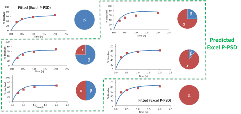
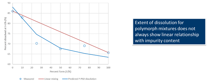
Data for Rifaximin from Dharani, S., et al. ²³ , show that the mixing law for percent dissolved at 2 hours for rifaximin form alpha and beta mixture is not linear and is well predicted using the P-PSD approach.

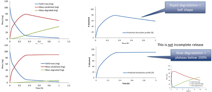
In case of degradation

When there is drug degradation in the medium, e.g. due to pH, the solubilized drug mass will be removed as time passes. This can accelerate the apparent drug dissolution and also lead to bell shaped profiles where the drug concentration in the vessel goes through a maximum and then diminish, or goes through an apparent plateau (if the dissolution balances the degradation).

The first order drug degradation rate constant can be used to calculate the mass degraded over time using the following equation, where  is the first order degradation rate constant, is the variation of mass degraded over the time interval  from time t, and is the drug mass solubilized at time t.

Equation 1-35: First-Order Drug Degradation Rate Equation