Tutorial: ADMET Predictor® Module
This tutorial explores the use of the optional ADMET Predictor® (AP) module which uses machine learning models to predict, from structure, the values of parameters e.g., solubility, pKa, logD, that are used in the pharmacokinetic (PK) simulations.
In this tutorial, we will cover:
Screening a database of compounds for fraction absorbed and bioavailability in human and rat
GPX™ can run batches of simulations from the Runs view to predict the Fa, bioavailability, Cmax, AUC, etc. for any number of compounds or scenarios. This project can be created either by manually entering information into GPX™ or by importing a file of molecular structures utilizing the AP module which will be the focus of this tutorial.
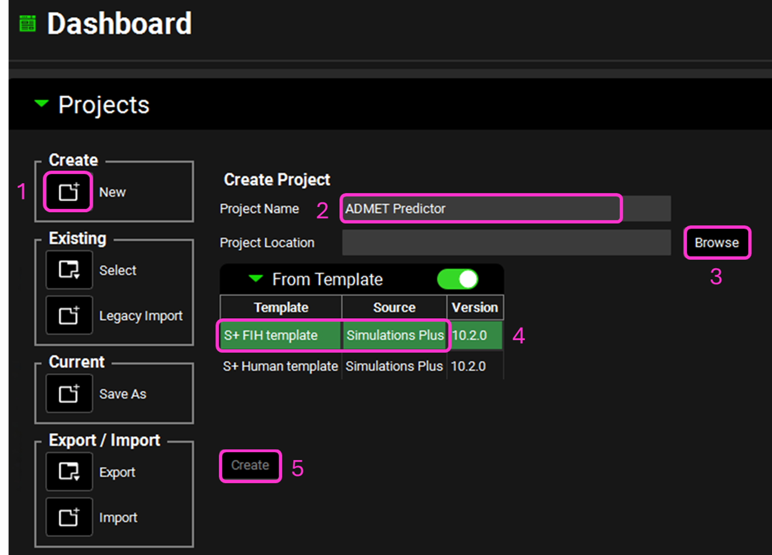
Open GPX™ and, in the Dashboard view, click on the icon next to New to create a New project.
Name the project “ADMET Predictor” by typing in the Project Name box and hitting Enter.
Click Browse and navigate to an existing folder (or create a new one) to store the project. Confirm your choice by clicking Select Folder.
Activate the toggle next to From Template and ensure the S+ FIH template is highlighted.
Click Create.
The template populates the project with some predefined Formulations, Dosing Schedules, and Physiologies.
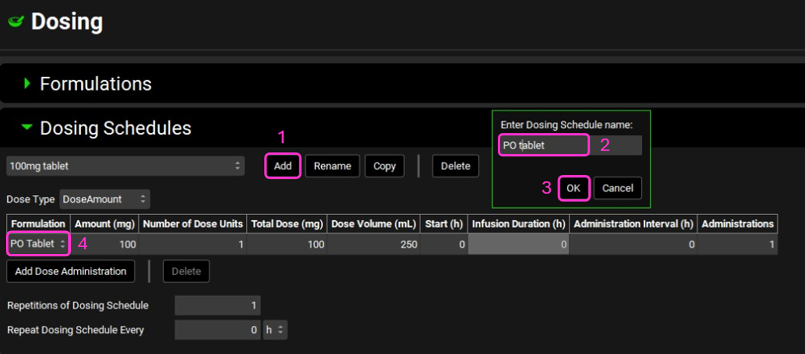
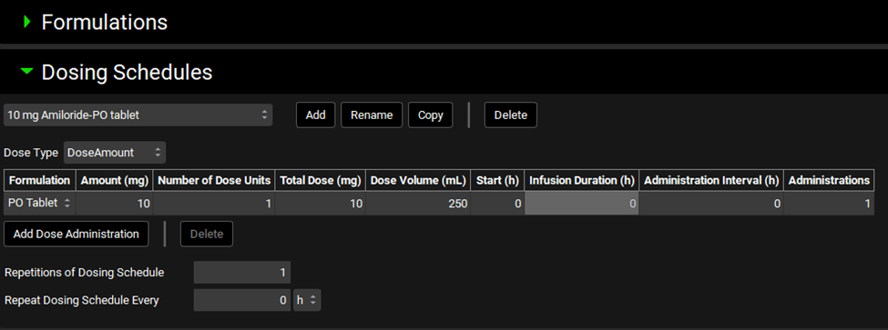
Navigate to the Dosing view and open the Dosing Schedules panel. Click Add and enter the name of the Dosing Schedule “PO Tablet” then click OK. Change the Formulation to PO Tablet and keep the other parameters as default.
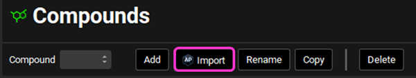
Navigate to the Compounds view. Now that we have populated the required assets for the ADMET Predictor® module we can import the compound structures. Go to the ADMET Predictor® module which can be accessed by either using the “AP Import” button in the Compounds panel or by clicking on ADMET Predictor® in the Modules pane on the right-hand side of the screen.
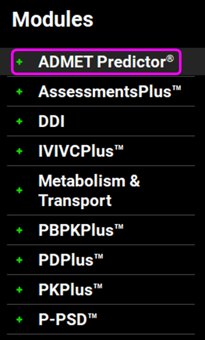
The modules list may differ from the screenshot, depending on which Modules are licensed. A green '+' sign indicates that a module is licensed (enabled), while a gray '+' sign indicates it is not.
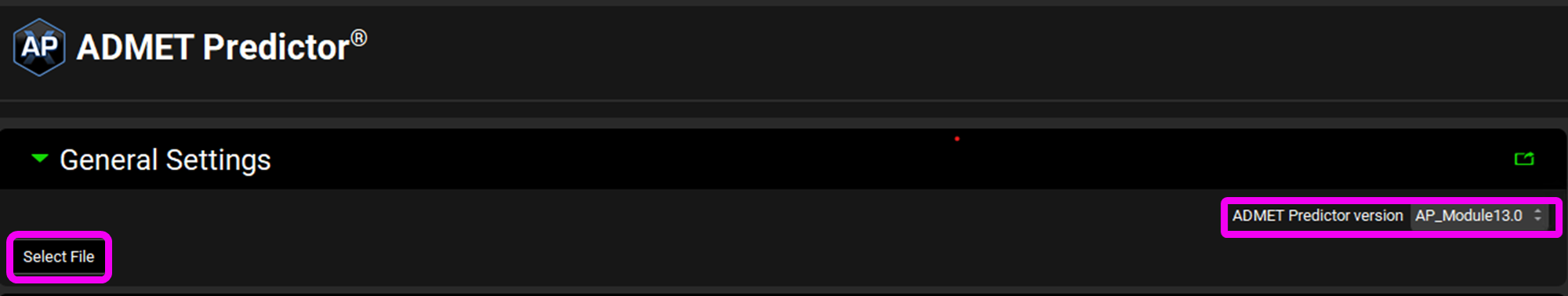
Click on “Select File” and navigate to the tutorials folder and in the 21-Comps-w-ExperData-3D folder, select the “21-Comps-w-ExperData-3D.sdf” file and click Open. You can see which AP version is being used on the right-hand side of the interface. AP_Module11.0 was released with GPX™ 10.1 whilst AP_Module13.0 was released with GPX™ 10.2.
The first import we will perform is for a PO tablet with a Human 30y 85.53kg Physiology Schedule. Click in the Dosing Schedule drop-down and select PO Tablet. Click in the Physiology Schedule drop-down and select Human 30y 85.53kg schedule. The Pharmacokinetic Model will be left as a Compartmental model. In the Pharmacokinetics table, if you license the AP Metabolism module, the Clearance model will default to Liver Microsomes which we will use.
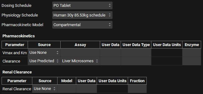
If you are licensing the PBPKPlus™ module, you could define a PBPK model along with an estimate of renal filtration clearance to be set up for all compounds. Switch the Pharmacokinetic Model to PBPK and the Renal Clearance Source will automatically switch to Use Predicted and the Model to Fup*GFR.
In addition, other models are available to predict clearance, including Hepatocytes. If you are licensing metabolism predictions via the ADMET Predictor® module along with the Metabolism and Transport module in GastroPlus®, you can select import of predicted Km and Vmax for CYP enzymes, or predicted total CL based on CYP enzyme metabolism.
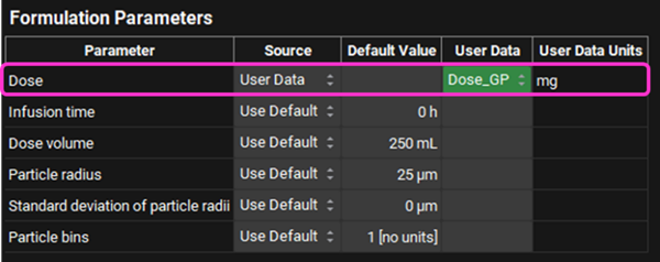
Expand the Advanced Settings panel. This opens up a list of parameters and enables you to specify columns in your .sdf file that contain data you wish to use in place of the AP predictions. The file we are using includes some measured data. Select “User Data” in the Source Column and the type of User Data for the Compound Name (found under General) and Dose (found under Formulation Parameters) as detailed below:

Once the appropriate selections have been made, scroll to the bottom of the window, and click Start Import.
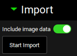
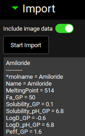
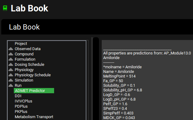
Once the program has finished importing all the compounds, the progress bar will disappear and information on the import will appear in the Log underneath the Start Import button, you may need to scroll down to see it. This information is also saved in the Lab Book in the “ADMET Predictor®” module.
Save the project by clicking on the Save button in the top right corner of the interface and clicking OK on the resulting Save completed box. Clear the information message in the Messages center indicating that for one compound the transcellular Peff is set to zero.
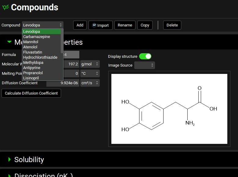
Navigate to the Compounds view using the navigation pane and see that the corresponding properties were predicted for each compound by expanding each panel/sub-panel. Changing the Compound in the drop-down underneath Compounds enables you to view the properties for each compound.
Navigate to the Dosing view using the navigation pane and then review the automatically created Dosing Schedules based on the dose specified for each compound in the .sdf.

If the automatically created dosing schedules are not visible (due to a refresh issue) you can add a new temporary dosing schedule (click add and then enter a single letter for the name), and it will refresh the list. You can then delete the temporary dosing schedule.
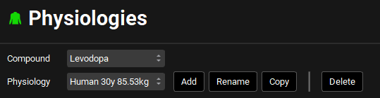
Navigate to the Physiologies view and ensure the physiology selected is Human 30y 85.53kg.
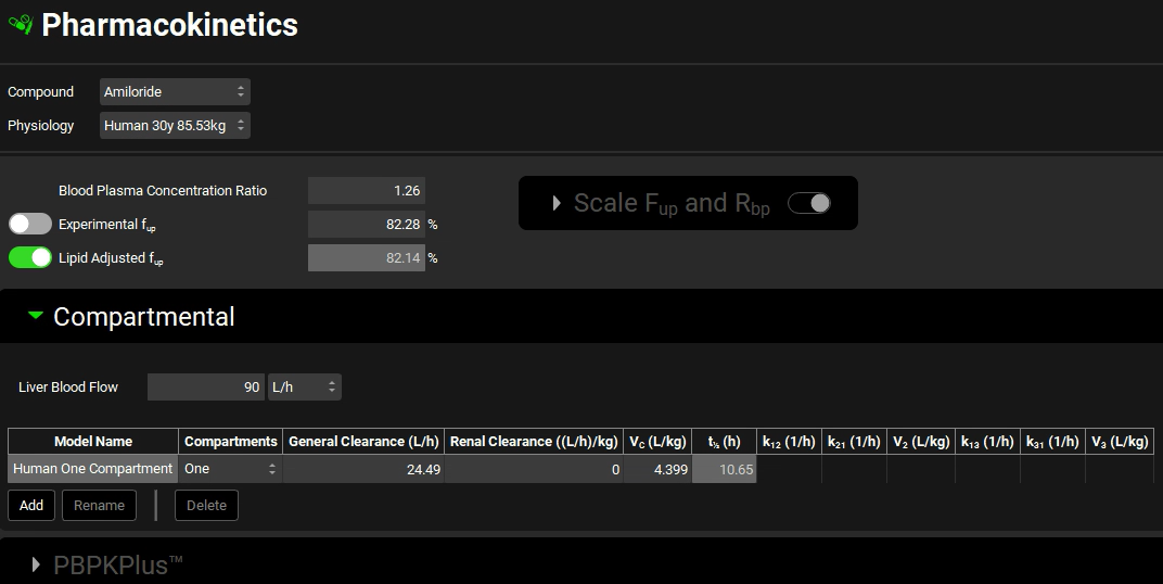
Navigate to the Pharmacokinetics view and review the pharmacokinetic parameters predicted for each compound by expanding the Compartmental panel and browsing through the different compounds using the drop-down list next to Compound at the top of the view.
If you imported using a PBPK model, the PBPKPlus™ panel will be active. Expanding the PBPKPlus™ panel and moving past the PBPK diagram to the table enables the clearance in the liver and the kidney to be seen in the CL column.
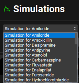
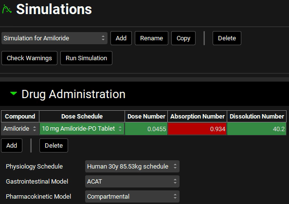
Navigate to the Simulations view. Notice that when ADMET Predictor® is used, a simulation is automatically created for each compound imported using the Dose Schedule, Physiology Schedule, and Pharmacokinetic Model specified during import. The message regarding the permeability of Amiloride will appear in the message center each time you navigate to that simulation.
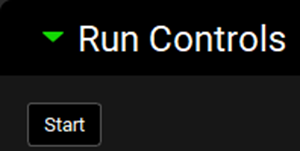
Navigate to the Runs view. Notice that there is a Run called Run, which, when you click on it, shows that the simulations for all compounds imported will be included in this run as all the toggle buttons in the Include column are turned on (indicated by the green color). Minimize the Output Settings panel by clicking on the green arrow or double clicking anywhere in the panel header bar. Click Start in the Run Controls panel at the bottom of the view.
When importing a structure through ADMET Predictor® a simulation is automatically created for each compound. Hence, you will see 21 simulations in this run corresponding to the 21 compounds.
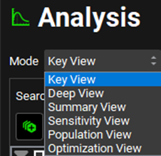
The Analysis View will automatically be activated when the Run has completed and will display the Key View Mode and the Cp-Time plot. Switch the Mode to Summary View by clicking in the Mode drop-down.
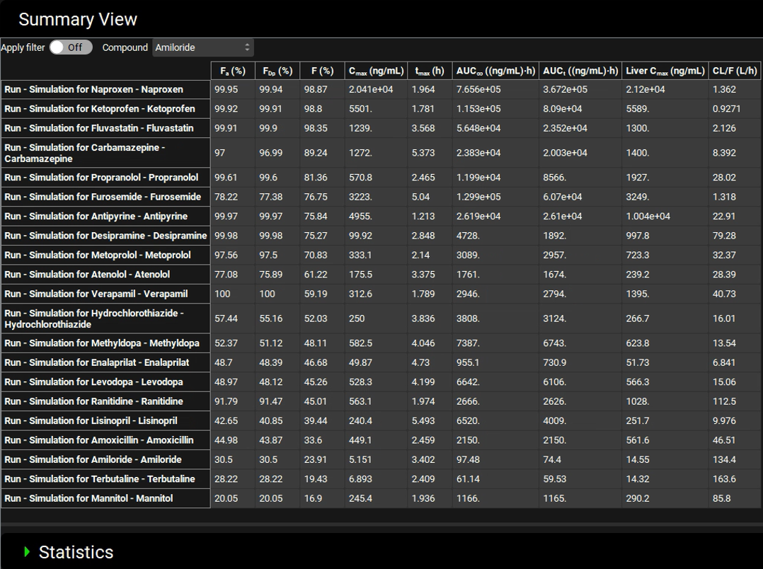
The Summary Table allows you to compare the Fa for all compounds in this project. You can sort the compounds from highest to lowest for any parameter, e.g. predicted Fa, bioavailability, AUC, etc. by holding down “Alt” key on your keyboard and left clicking the parameter of interest on the column header. As there is no observed data associated with these simulations the Observed data on toggle can be turned off to remove the observed columns. The toggle will turn grey and will be renamed Observed data off. The length of the summary table can be increased by hovering over the dividing line between the table and the Statistics panel, so that the cursor changes to a double arrow, then left click on the mouse and drag it to the down until all rows are visible.
It can be seen that Naproxen has the highest F(%). To determine whether this is also the case for an oral suspension dose in rat we can import the compounds for a second time, this time using rat predictions for parameters such as fraction unbound in plasma, microsomal clearance, and blood to plasma ratio.
Navigate to the ADMET Predictor® Module by clicking on ADMET Predictor® in the Modules pane.
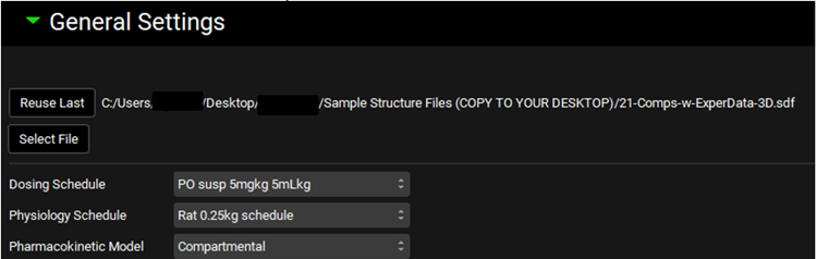
Adjust the Dosing Schedule to “PO susp 5mgkg 5mLkg” to dose a 5 mg/kg oral suspension dose using a dose volume of 5 mL/kg.
Adjust the Physiology Schedule to Rat 0.25kg schedule.
Open the Advanced Settings panel and set the Source for the Dose (in the Formulation Parameters table) to Use Default.
Save the project and click OK.
Scroll to the bottom of the ADMET Predictor® view and click the Start Import button in the Import panel.
Once the program has finished importing all the compounds, the progress bar will disappear and information on the import will appear in the Log underneath the Start Import button.
Save the project and click OK.
Navigate to the Compounds view and click on the Compound drop-down to see that additional compounds have been added, each with a suffix of 1.
Navigate to the Physiologies view and select “Verapamil1” and “Rat 0.25kg” as the Compound and the Physiology.
Navigate to the Pharmacokinetics view, expand the Compartmental panel (if necessary), and note that the Model Name is Rat One Compartment.
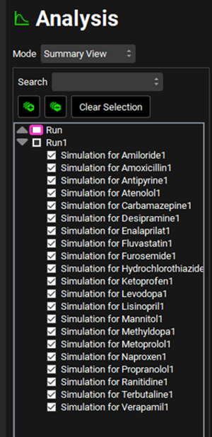
Navigate to the Runs view. A second Run has been created called Run1 – note that this contains all the Simulations for Compounds with the suffix of 1.
Minimize the Output Settings and click Start under the Run Controls panel.
The Analysis View will automatically be activated when the Run has completed and will display the Key View Mode and the Cp-Time plot. Switch the Mode to Summary View by clicking in the Mode drop-down.
Hold down “Alt” key on your keyboard and left clicking the F(%) column header. It can be seen that the compound with the highest bioavailability in the rat (at a 5 mg/kg dose) is Fluvastatin. Naproxen is 2nd in the table with a bioavailability of 96.54%.
Note that on the left side of the summary table is a list of simulations. The simulations from the first Run can be added to the summary table by checking the box next to the Run name allowing you to compare the Summary parameters for all compounds and scenarios.