Tutorial: DDI Module

The DDI Module in GastroPlus® includes prediction of competitive inhibition, time-dependent inhibition, and induction of enzymes and transporters under steady-state assumptions as well as full dynamic simulations. This tutorial provides several step-by-step examples guiding you through the process of obtaining the fm values (the fraction of substrate’s clearance due to each specific enzyme) from in vitro data, producing simple steady-state predictions of DDI potential, and obtaining the DDI predictions from full dynamic simulations.

In this tutorial, we will cover:

• fm calculation from in vitro data using recombinant enzymes

• fm calculation from in vitro data in human liver microsomes

• Dynamic DDI

fm calculation from in vitro data using recombinant enzymes

Transforming the information obtained from in vitro assays with recombinant CYP enzymes (rCYP) into the fm values in a specific population and applying them in a steady-state DDI prediction.

The metabolic profile using rCYPs is assessed by measuring in vitro clearance of the test compound using a system expressing one CYP enzyme at a time. The specific activity of the recombinant CYP enzyme may differ from the specific activity of the same CYP enzyme in vivo and these differences are commonly accounted for through intersystem extrapolation factors (ISEFs). ISEF values may be obtained from in vitro clearances of standard substrates for corresponding CYP enzymes measured in human liver microsomes (HLM) and in the same rCYP system that was used to assay the test compound.

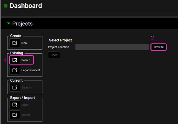
1. Open GPX™ and, in the Dashboard view, click on the icon next to Select to open an Existing project.

2. Click Browse and navigate to the C:\Users\<user>\AppData\Local\Simulations Plus, Inc\GastroPlus\10.2\Tutorials\Ketoconazole folder and select the project file Ketoconazole.gpproject by clicking on it and clicking Open.

3. Click on the Compounds view in the navigation pane, then click on Add, enter the name “Drug 1 rCYP” and click on OK (or press Enter). We will use the default properties.

4. Click on the Dosing view in the navigation pane and expand the Formulations panel, by clicking on the green arrow or double clicking on the panel header bar, and check that there is a formulation called “IR Tablet 5um”.

5. Expand the Dosing Schedules panel and click on Add. Enter “100mg IR Tablet 5um” as the Dosing Schedule name and click on OK. Note that the default Amount is 100 mg.

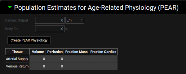
6. Click on the Physiologies view in the navigation pane to see the Physiology “Human 70kg Fasted”. If you have the PBPKPlus™ module license, expand the Population Estimates for Age-Related Physiology (PEAR) panel to confirm that no PEAR physiology has been created (if the PBPKPlus™ module is not licensed, the panel will be disabled).

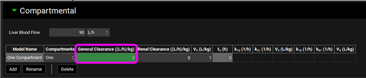
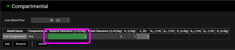
7. Click on the Pharmacokinetics view in the navigation pane, check that the Compound is “Drug 1 rCYP” and expand the Compartmental panel. Change the General Clearance to 0 L/h/kg and press Enter.

8. Click on the Simulations view in the navigation pane and then click on Add. Enter the Simulation name “100mg Tablet Drug 1 rCYP” and click on OK. Change the Compound to “Drug 1 rCYP” and the Dose Schedule to “100mg IR Tablet 5um”. A caution message will appear. Click on Done to delete it. Save the project, using the button in the top right corner of the interface, and click on OK.

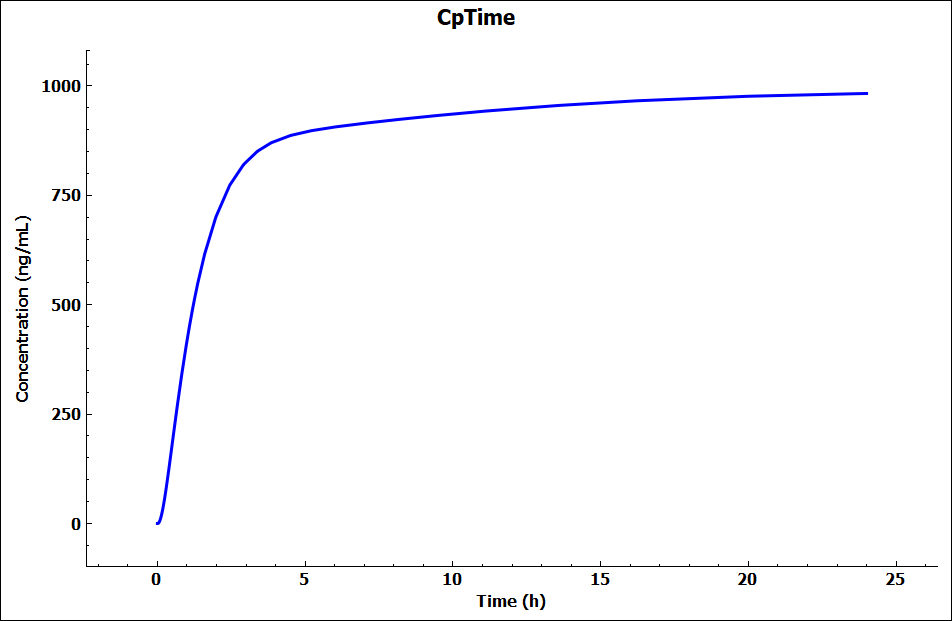
9. Click on Check Warnings and then Run Simulation (both buttons are towards the top of the Simulations view). When the simulation completes the interface will automatically switch to the Analysis view, displaying the C_p-Time plot from the Key View Mode. The C_p-Time profile highlights there is no clearance in the model.

10. Click on DDI in the Modules pane on the right-hand side of the interface.

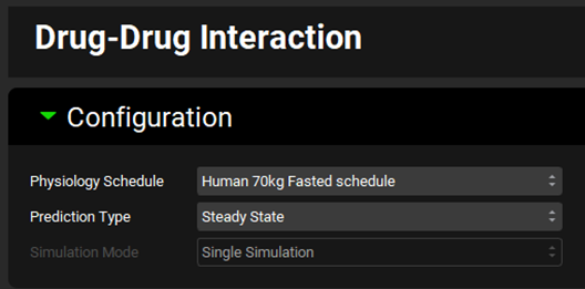
11. Expand the Configuration panel to see the Physiology Schedule “Human 70kg Fasted Schedule” has been automatically selected and leave the Prediction Type as “Steady-State”.

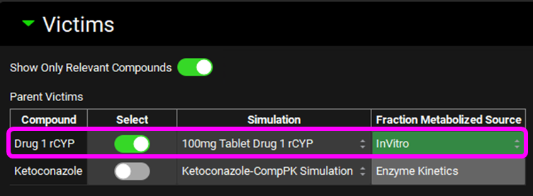
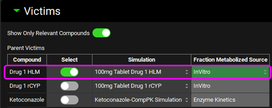
12. Expand the Victims panel and Select, via the toggle, the Compound “Drug 1 rCYP” before switching the Fraction Metabolized Source to “InVitro”.

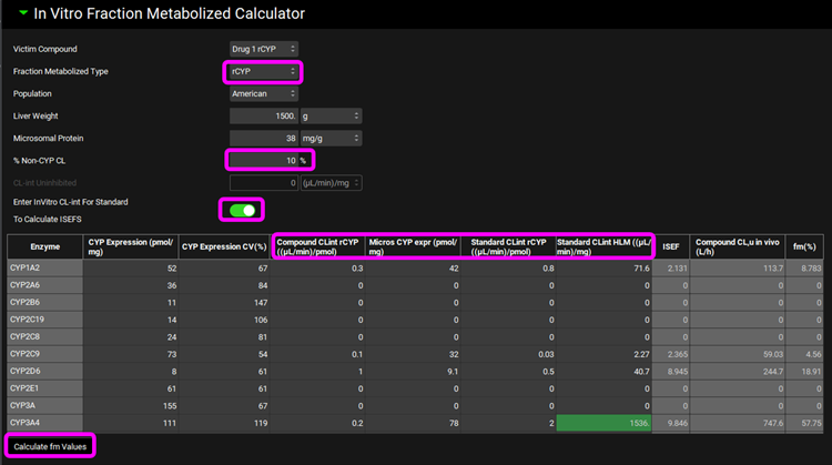
13. Scroll down and expand the In Vitro Fraction Metabolized Calculator sub-panel. Select “rCYP” as the Fraction Metabolized Type, enter 10% for % Non-CYP CL and press Enter, set the toggle on for Enter InVitro CL-int For Standard To Calculate ISEFS, enter the data in the tables below and then click on Calculate fm Values. The Tab key can be used to move across the rows in the table to enter the data.

14. Scroll down and expand the Perpetrators panel, turn the toggle off for Show Only Relevant Perpetrators and Select, via the toggle, the Compound “Ketoconazole”.

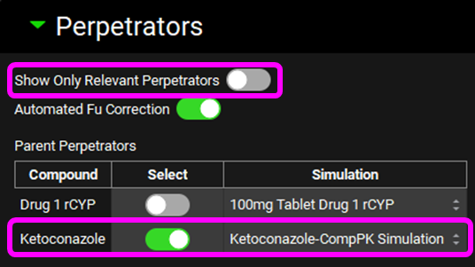
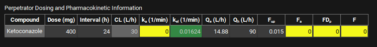
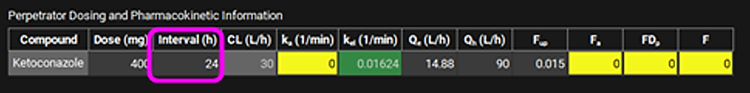
15. Scroll down and enter a 400 mg Dose and an Interval of 24 h for Ketoconazole in the Perpetrator Dosing and Pharmacokinetic Information table.

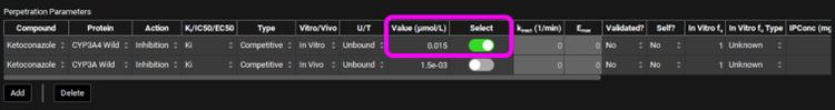
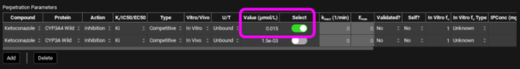
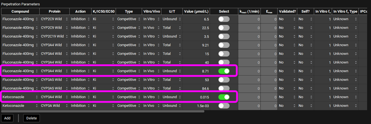
16. Select, via the toggle, an inhibition constant of 0.015 µmol/L for CYP3A4 in the Perpetration Parameters table.

17. Save the project and click on OK.

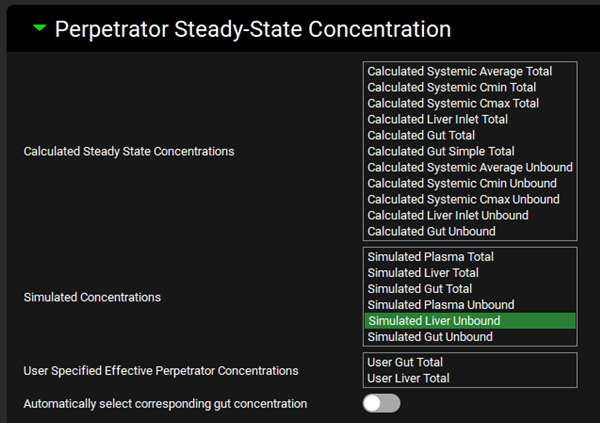
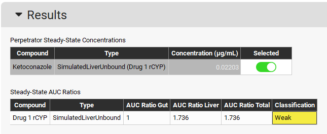
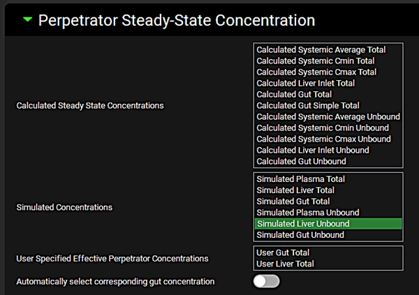
18. Expand the Perpetrator Steady-State Concentration panel and select Simulated Liver Unbound in the Simulated Concentrations box.

19. Expand the Run panel, click on Check Warnings, click on Done on the message appearing at the top in the message section, and then click on Steady-State Prediction.

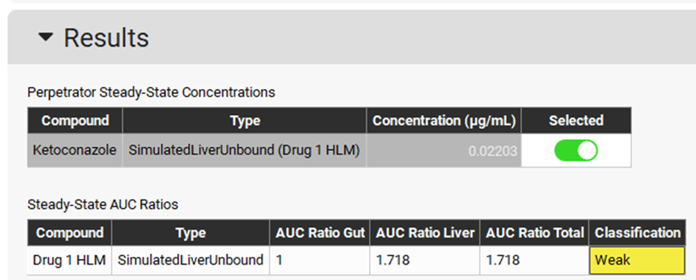
20. When the Run Controls panel disappears, scroll down to the Results panel, which will automatically expand when the predictions have been made, and see that a Weak interaction is predicted.

fm calculation from in vitro data in human liver microsomes

In this example we will guide you through the process of transforming the information obtained from in vitro assays with human liver microsomes (HLM) into the fm values (fractions of total clearance due to each specific enzyme) in a specific population and applying them in a steady-state DDI prediction.

The metabolic profile using HLM is assessed by using specific inhibitors of individual CYP enzymes.

1. Open GPX™ and, in the Dashboard view, click on the icon next to Select to open an Existing project.

2. Click Browse and navigate to the C:\Users\<user>\AppData\Local\Simulations Plus, Inc\GastroPlus\10.2\Tutorials\Ketoconazole folder and select the project file Ketoconazole.gpproject by clicking on it and clicking Open, if not already open.

3. Click on Compounds in the navigation pane, then click on Add, enter the name “Drug 1 HLM” and click on OK (or press Enter). We will use the default properties.

4. Click on Dosing in the navigation pane and expand the Dosing Schedules panel, by clicking on the green arrow or double clicking on the panel header bar, and, if you have not completed the fm calculation from recombinant enzyme data tutorial, click on Add. Enter “100mg IR Tablet 5um” as the Dosing Schedule name and click on OK. Note that the default Amount is 100 mg.

5. Click on Physiologies in the navigation pane to see the Physiology “Human 70kg Fasted” and expand the Population Estimates for Age-Related Physiology (PEAR) panel to confirm that no PEAR physiology has been created.

6. Click on Pharmacokinetics in the navigation pane, check that the Compound is “Drug 1 HLM” and expand the Compartmental panel. Change the General Clearance to 0 L/h/kg and press Enter.

7. Click on Simulations in the navigation pane and then click on Add. Enter the Simulation name “100mg Tablet Drug 1 HLM” and click on OK. Change the Compound to “Drug 1 HLM” and the Dose Schedule to “100mg IR Tablet 5um”. Save the project, using the button in the top right corner of the interface, and click on OK.

8. Click on Check Warnings and then Run Simulation (both buttons are towards the top of the Simulations view). When the simulation completes the interface will automatically switch to the Analysis view, displaying the C_p-Time plot from the Key View Mode. The C_p-Time profile highlights there is no clearance in the model.

9. Click on DDI in the Modules pane on the right-hand side of the interface.

10. Expand the Configuration panel to see the Physiology Schedule “Human 70kg Fasted Schedule” has been automatically selected and leave the Prediction Type as “Steady-State”.

11. Expand the Victims panel and Select, via the toggle, the Compound “Drug 1 HLM” before switching the Fraction Metabolized Source to “InVitro”.

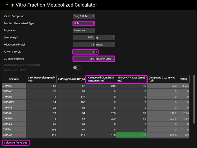
12. Scroll down and expand the In Vitro Fraction Metabolized Calculator sub-panel. Select “HLM” as the Fraction Metabolized Type, enter 10% for % Non-CYP CL and press Enter, enter 269 µL/min/mg for CL-int Uninhibited and press Enter, enter the data in the table below and then click on Calculate fm Values. The Tab key can be used to move across the rows in the table to enter the data.

This step may be completed with the panel popped out, using the icon on the panel header bar. To pop the panel back in, click the “x” in the top right corner of the Invitro Fraction Metabolized Calculator window.

13. Scroll down and expand the Perpetrators panel, if necessary, turn the toggle off for Show Only Relevant Perpetrators and Select, via the toggle, the Compound “Ketoconazole”.

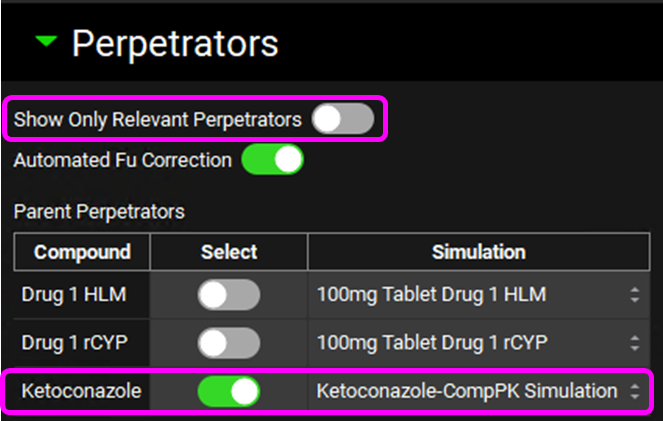
14. Scroll down and enter a Dose of 400 mg and an Interval of 24 h for Ketoconazole in the Perpetrator Dosing and Pharmacokinetic Information table and press Enter.

15. Select, via the toggle, an inhibition constant of 0.015 µmol/L for CYP3A4 in the Perpetration Parameters table.

16. Save the project and click on OK.

17. Expand the Perpetrator Steady-State Concentration panel and select Simulated Liver Unbound.

18. Expand the Run panel, click on Check Warnings and then click on Steady-State Prediction.

19. When the Run Controls panel disappears, scroll down to the Results panel, which will automatically expand when the predictions have been made, and see that there is predicted to be a Weak interaction.

Dynamic DDI

Part 1: Midazolam-Ketoconazole interaction

In this example we will work on a prediction of a competitive midazolam-ketoconazole interaction. The main route of elimination for these two compounds is metabolism by CYP3A4 and their coadministration may potentially result in a significant increase in exposure of either one or both compounds.

1. Open GPX™ and, in the Dashboard view, click on the icon next to Select to open an Existing project.

2. Click Browse and navigate to the C:\Users\<user>\AppData\Local\Simulations Plus, Inc\GastroPlus\10.2\Tutorials\Dynamic DDI folder and select the project file Dynamic DDI.gpproject by clicking on it and clicking Open.

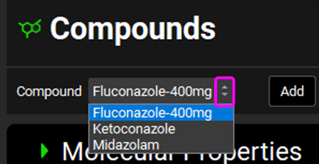
3. Click on Compounds in the navigation pane and then click on the Compound drop-down selector to see that there are three compounds in this project.

4. Click on Physiologies in the navigation pane to see the Physiology "Human 70kg Fasted" and expand the Population Estimates for Age-Related Physiology (PEAR) panel, by clicking on the green arrow or double clicking on the panel header bar, to confirm that no PEAR physiology has been created.

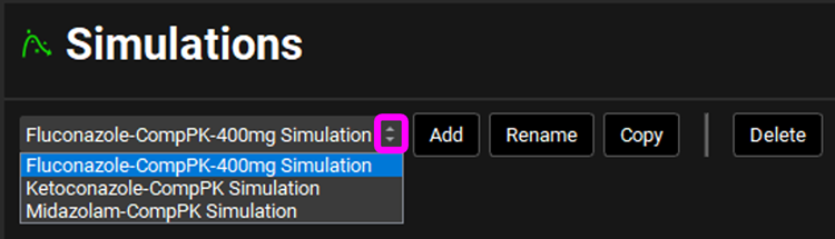
5. Click on Simulations in the navigation pane and then click on the drop-down selector to see that there are three simulations in this project, as for a DDI prediction there must be a simulation for each compound (victim or perpetrator).

6. Click on DDI in the Modules pane on the right-hand side of the interface.

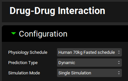
7. Expand the Configuration panel to see the Physiology Schedule “Human 70kg Fasted Schedule” has been automatically selected and switch the Prediction Type to “Dynamic”. Leave the Simulation Mode as “Single Simulation”.

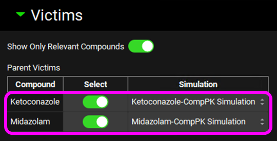
8. Expand the Victims panel and Select, via the toggles, the Compounds “Ketoconazole” and “Midazolam”.

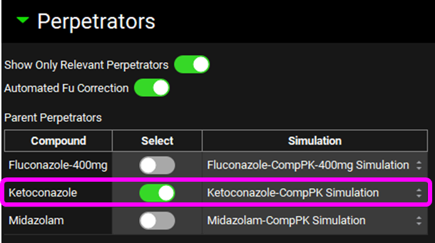
9. Scroll down and expand the Perpetrators panel and Select, via the toggle, the Compound “Ketoconazole”.

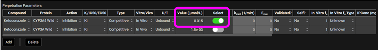
10. Select, via the toggle, an inhibition constant of 0.015 µmol/L for CYP3A4 in the Perpetration Parameters table.

11. Save the project, using the button in the top right corner of the interface, and click on OK.

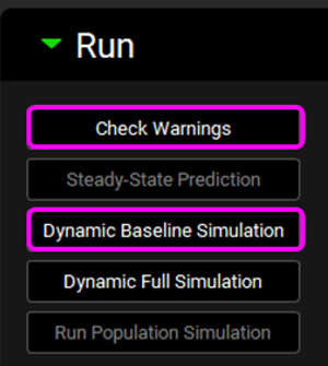
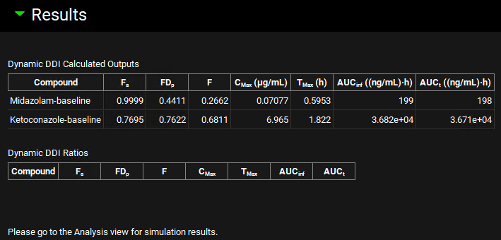
12. Scroll down and expand the Run panel, click on Check Warnings, and then click on Dynamic Baseline Simulation.

13. When the Run Controls panel disappears, scroll down to the Results panel, which will automatically expand when the predictions have been made, and assess the baseline predictions of pharmacokinetic parameters.

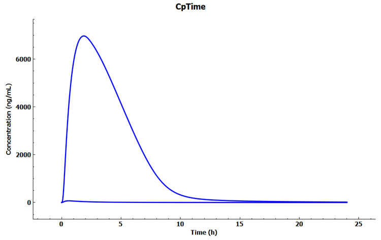
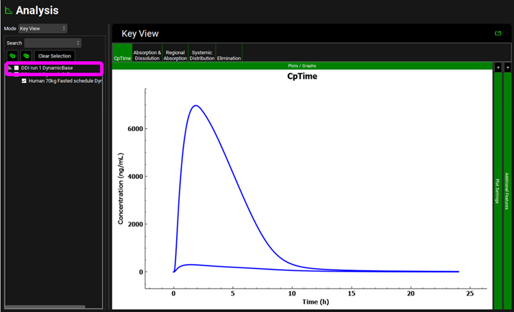
14. Click on Analysis in the navigation pane to see the C_p-Time Key View plot for the baseline simulation.

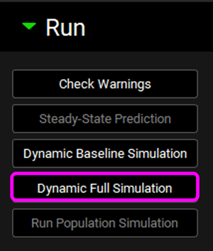
15. Click on DDI in the Modules pane and then click on Dynamic Full Simulation in the Run panel.

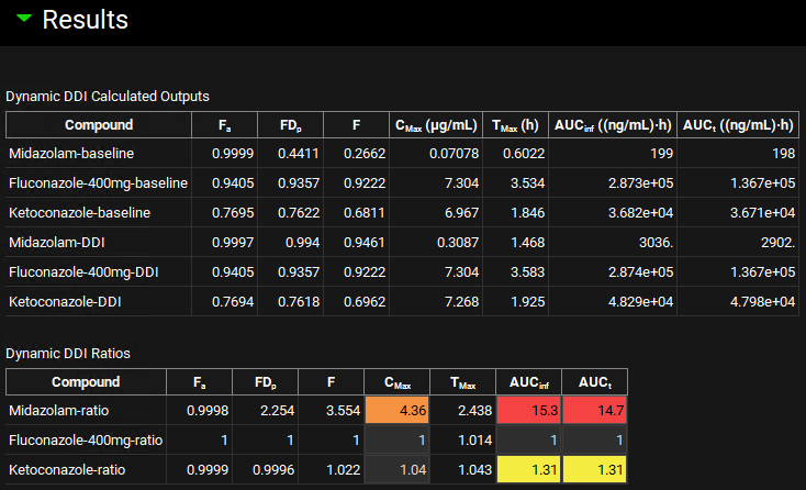
16. When the Run Controls panel disappears, scroll down to the Results panel, and assess the DDI predictions of pharmacokinetic parameters and DDI ratios.

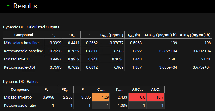
The ratio of results from full and baseline simulation for each compound is highlighted in yellow (weak interaction), orange (moderate interaction), or red (strong interaction) for easy identification of the magnitude of DDI.

17. Click on Analysis in the navigation pane to see the C_p-Time Key View plot for the dynamic simulation. Note that you can reselect the baseline C_p-Time Simulation in the simulation list. Expand the “DDI run 1 DynamicBase” by clicking the arrow and then check the box next to “Human 70kg Fasted schedule DynamicBase”.

Part 2: Midazolam-Ketoconazole-Fluconazole interaction

In GPX™ it is possible to simulate polypharmacy and include an unlimited number of compounds, both victims and perpetrators. Let’s add fluconazole, a CYP3A4 inhibitor, to the simulation.

1. Click on DDI in the Modules pane, scroll back up to the Perpetrators panel and Select, via the toggle, the Compound "Fluconazole-400mg". Leave “Ketoconazole” selected.

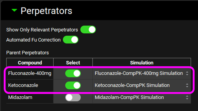
2. Select, via the toggle, an inhibition constant of 8.71 µmol/L for CYP3A4 for” Fluconazole-400mg” in the Perpetration Parameters table. Leave the “Ketoconazole” selection as is.

3. Scroll down and click on Dynamic Baseline Simulation in the Run panel. When the Run Controls panel disappears, scroll down to the Results panel, and assess the baseline predictions of pharmacokinetic parameters. Note: If you click on Check Warnings then a message will appear in the Messages center to say In vivo perpetration(s) were selected for Dynamic DDI. Click on Done after you have read the message.

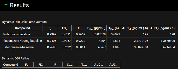
4. Click on Dynamic Full Simulation in the Run panel. When the Run Controls panel disappears, scroll down to the Results panel, and assess the DDI predictions of pharmacokinetic parameters and DDI ratios. Note the increased DDI ratios for both Midazolam and Ketoconazole.

Part 3: DDI Population Simulation

Within GPX™ it is possible to simulate DDI predictions for populations of subjects. Let’s run a population simulation for the midazolam-ketoconazole-fluconazole interaction.

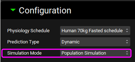
1. Within the DDI module scroll up to the Configuration panel and select “Population Simulation” as the Simulation Mode.

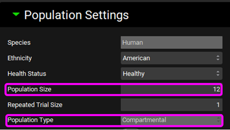
2. Scroll down to the Populations Settings panel, which will now be enabled, and expand it. Enter a Population Size of “12” and make sure the Population Type is set to “Compartmental”.

3. Save the project and click OK.

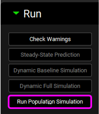
4. Scroll down to the Run panel and click on Run Population Simulation.

5. When the Run Controls panel disappears, scroll down to the Results panel, and assess the DDI predictions of pharmacokinetic parameters and DDI ratios. Use the Compound drop-down list selector to review the population predictions for each compound.

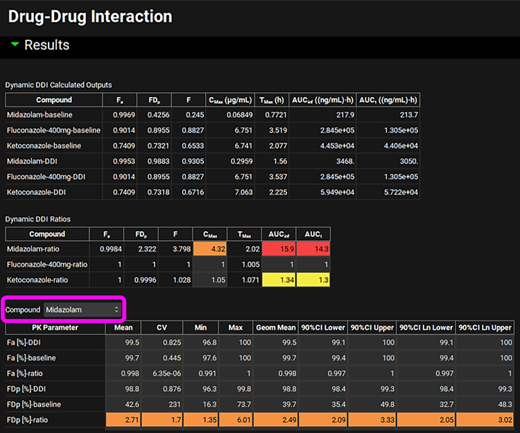
Because Population Simulator is based on random samples, results will likely differ from the results shown in the previous figure.

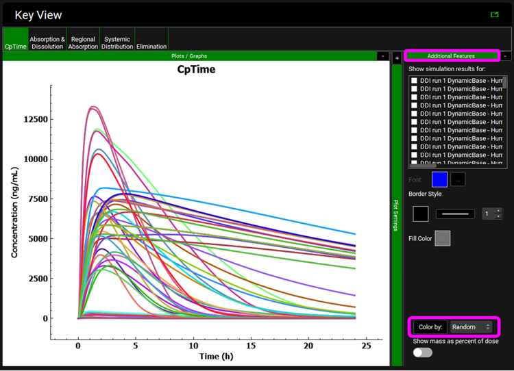
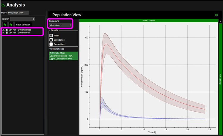
6. Click on Analysis in the navigation pane to go to the Population View Mode. Via the simulation list select which population simulations you would like to view. Within the Population View panel use the Compound drop-down list selector to view the population predictions for each compound.

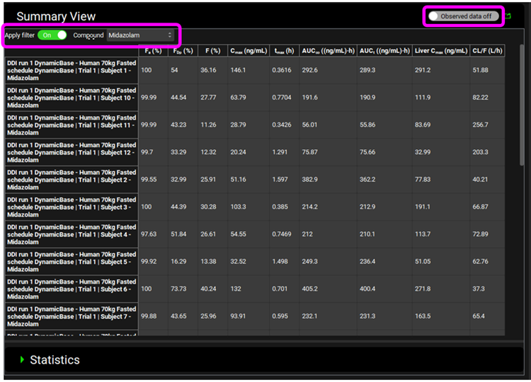
7. Within the Analysis view you can switch the Mode to Summary View to see the prediction of parameters and statistics for the individual subjects. You can Apply filter to focus on one compound and set the Observed data toggle to off to view all predicted parameters without having to scroll across.

Population Simulation files are automatically created for baseline and full simulations and are saved in folders within the folder containing the GPX™ project.

8. Within the Analysis view you can switch the Mode to Key View to see the C_p-Time profiles for each subject.

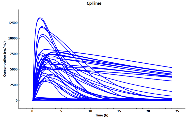
9. Expand Additional Features via "+", change to Random in the drop-down list and then click on Color by to randomly color each curve.