Tutorial: GPX™ Run Modes and Loading Observed Data
In this tutorial, we will cover:
Opening the GPX™ project and familiarization with the assets
Linking Observed Data Profiles and Parameters with Simulations
Running the Simulations (individually and as a batch) and viewing the results
Opening the GPX™ project and familiarization with the assets
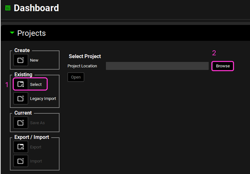
Open GPX™ and, in the Dashboard view, click on the icon next to Select to open an Existing project.
Click Browse and navigate to the C:\Users\<user>\AppData\Local\Simulations Plus, Inc\GastroPlus\10.2\Tutorials\GPX Run Modes and select the project file GPX Run Modes.gpproject by clicking on it and clicking open.
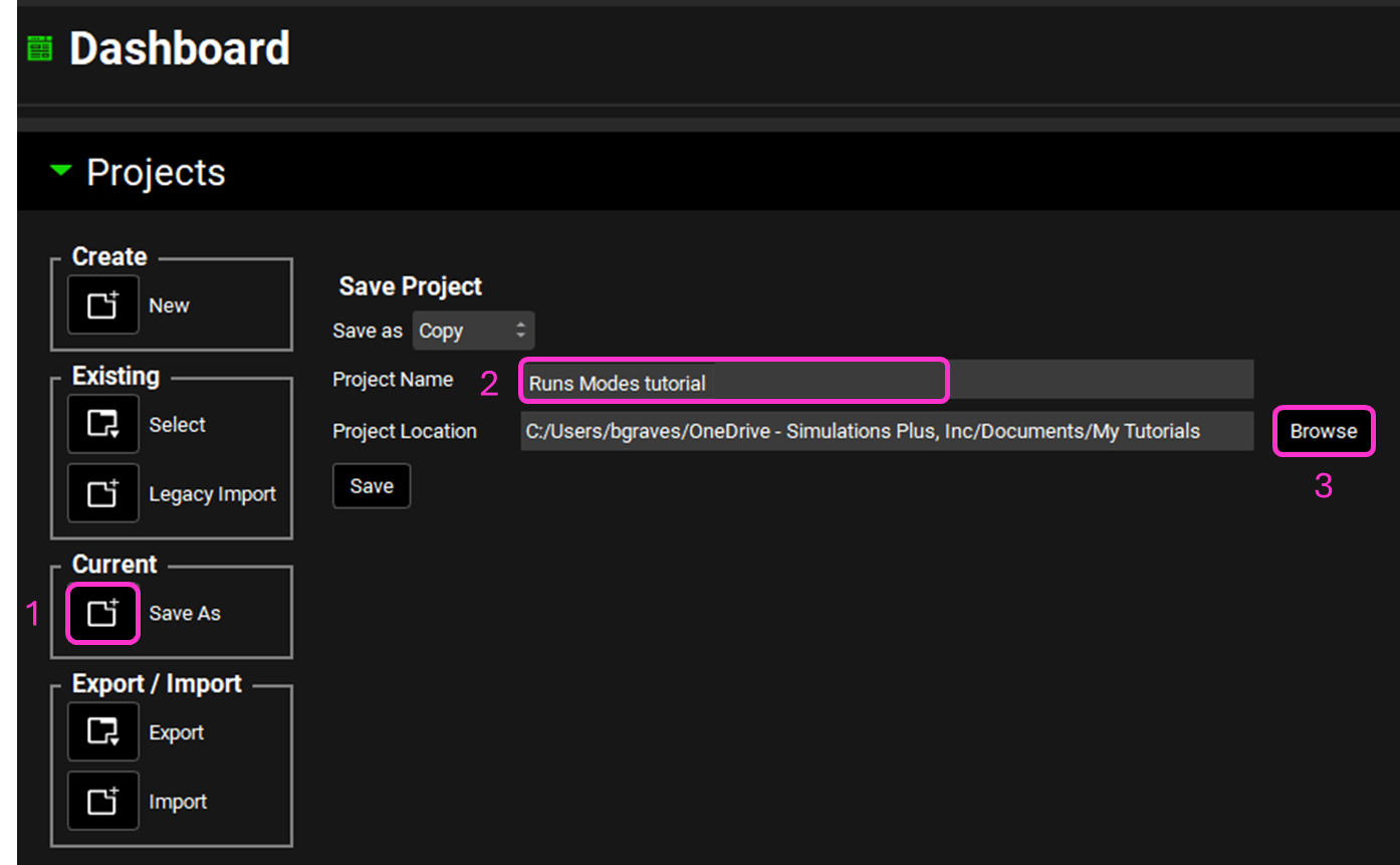
Now we will save a copy of the project to keep the original project unaltered. In the Dashboard view, click on the icon next to Save As under the Current frame. From the Save as drop-down, select Copy. Type “Runs Modes tutorial” as the Project name and click Browse to navigate to/add a folder to Save the project in. Click Save - you will see an information message in the Messages Center indicating that the project has been successfully copied. This message will disappear once you click 'Yes' on the pop-up window that also appears.
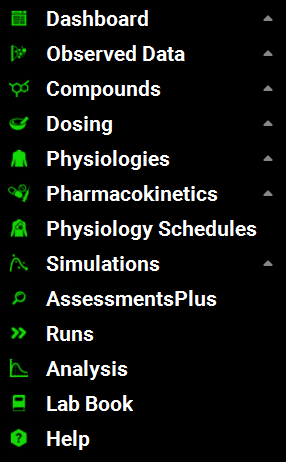
Move through the views on the navigation pane from Compounds to Simulations, observing the information that has been entered in this project.

In the Compounds view you can review the input parameters for each of the 9 compounds. The Dosing view displays the different formulations and schedules dosed in this project. In the Physiologies view you will see information that is not specific for each compound, but instead is specific for the demographics of the human subject used. The Pharmacokinetics view pairs a compound with a physiology and displays the physiomolecular properties and the compartmental pharmacokinetics for each compound. The Physiology Schedules view lists the physiologies that will be used throughout the dosing period. The Simulations view combines the reusable assets and the simulation settings to define which will be used in each simulation.
Loading Observed Data Profiles and Parameters
To add plasma concentration versus time (Cp-Time) data:
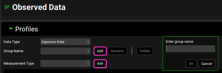
Move to the Observed Data view and ensure Exposure Data is selected as the Data Type.Click “Add” next to the Group Name and type Propranolol HCl PO 160mg in the pop-up box for the group name then click OK.
Ensure the Measurement Type is Concentration and click “Add” then type Cp-Time in the pop-up box for the series name and click OK.
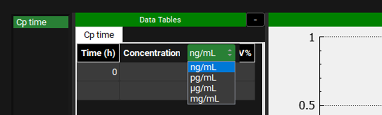
Check the correct units are displayed in the Time (h) and the Concentration (ng/mL) columns of the data table. To change the units, click on the unit in the column header and select the appropriate one from the list.
Open the Input Data for GPX Run Modes.xlsx and copy the Propranolol Cp-Time data found on the PO Cp time tab. Move to GPX and paste the data by right clicking in the first cell of the Time column and selecting Paste. The plot should be enabled displaying the observed data and the error bars.
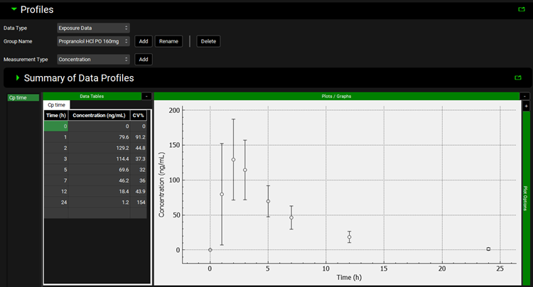

Ensure the correct units are selected in the column headers before pasting your data. If data is entered first and units are changed afterward, the program will automatically convert the values based on the newly selected units, which may lead to incorrect data representation.
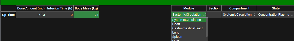
Scroll down to the table beneath the plot and fill in the following information:
Dose Amount (mg) 140.28; Body Mass (kg) 74
The right-hand side of the table maps the data to enable the program to recognize the type of data entered and plot it against the correct simulated curve so click in each box and select the following:
Module: Systemic Circulation; Compartment: Systemic Circulation; State: Concentration Plasma
Repeat steps 1 to 6 for Piroxicam
Group Name: Piroxicam 20mg
Series Name: Cp-Time
Ensure the correct units are selected before pasting your data: Time (h) and Concentration (µg/mL) – adjust them by clicking on the unit in the column header and selecting the correct one from the list.
Dose Amount (mg) 20; Body Mass (kg) 78
Module: Systemic Circulation; Compartment: Systemic Circulation; State: Concentration Plasma
Save the project.

Close the Profiles panel by clicking on the green arrow or double clicking on the panel bar and open the Parameters panel – this table allows you to enter observed PK parameters for the data that you have.
Click Add and type in Propranolol HCl 160mg PO tablet before pressing OK.
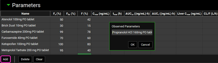
Click Add again and type in Piroxicam 20mg PO capsule before pressing OK.
Locate the rows you have just added in the table (you may have to scroll down to see them)
Enter the observed parameters that are found in the Input Data for GPX Run Modes.xlsx on the Parameters tab by clicking in the appropriate cells.
Save the project.
Linking Observed Data Profiles and Parameters with Simulations
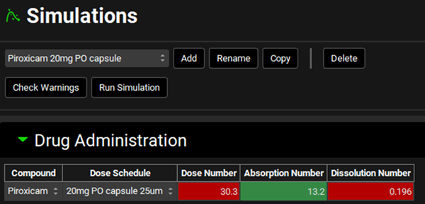
Move to the Simulations view, select the Piroxicam 20mg PO capsule as the simulation and notice the color of the text boxes for Dose Number, Absorption Number, and Dissolution Number (in the Drug Administration panel). The colors change depending on the physicochemical and biopharmaceutical properties of the drug selected and approximate when a drug molecule is likely to change to a different one of the four Biopharmaceutical Classification System (BCS) categories. All green indicates high solubility, high permeability, and rapid dissolution. Red absorption number and green dose number indicates high solubility and low permeability (probably BCS Class III), etc. These categories are not perfect cutoffs for the BCS as defined by the FDA, but they correctly represent most drugs.
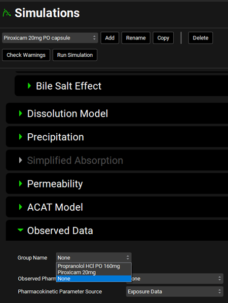
Expand the Compound Settings panel, scroll down to the Observed Data sub-panel and expand it. Select Piroxicam 20mg as the group name and Piroxicam 20mg PO capsule as the Observed PK Parameters. For the Pharmacokinetic Parameter Source choose either Exposure data (if you want the parameters to be calculated from the Cp-Time profile) or Parameters (if you want the entered PK parameters to be displayed). For this example, we will select Exposure Data.
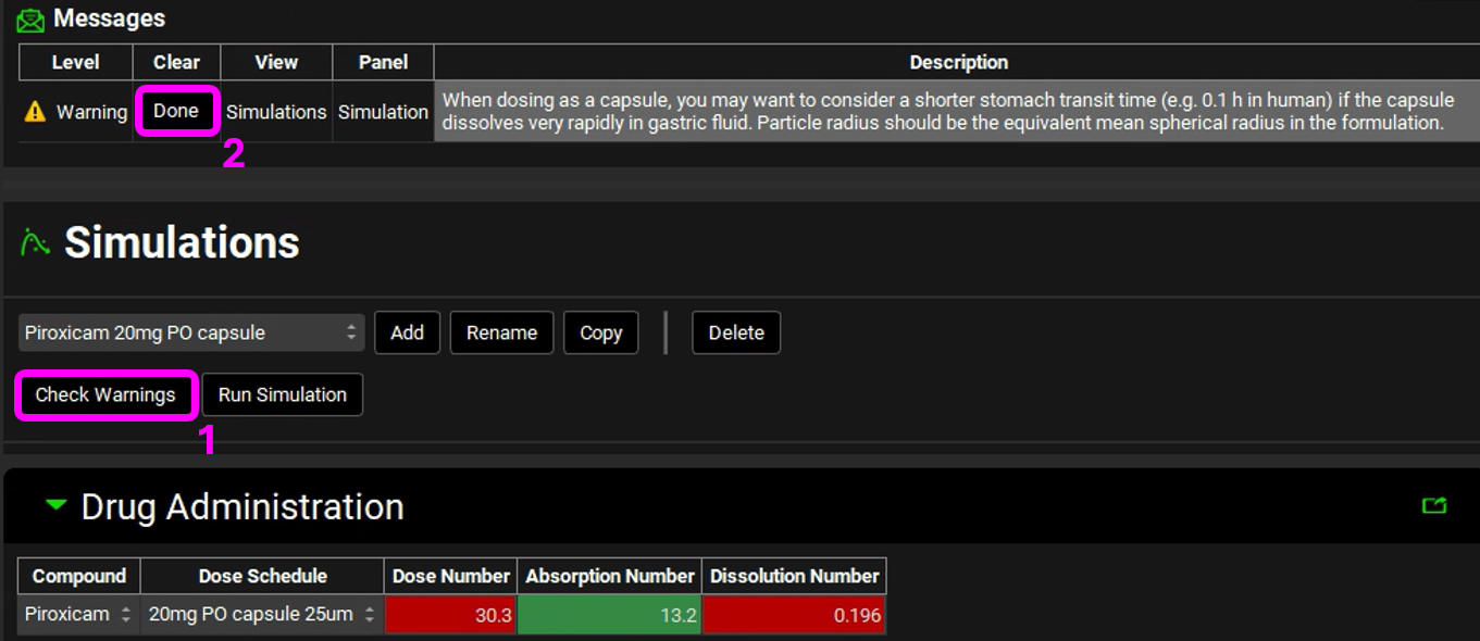
Click on the Check Warnings button (located at the top of the view underneath the Simulation selection area) and note the Warning that appears in the message center about reducing stomach transit time as the dose formulation is a capsule. For this example, we will continue without adjusting it. Click the Done button in the message center to remove the warning.
Switch the simulation to Propranolol HCl PO 160mg tablet and in the Observed Data sub-panel set the Group Name as Propranolol HCl PO 160mg, the Observed PK Parameters as Propranolol HCl 160mg PO tablet and the PK Parameter Source as Parameters.
Save the project.
Running the Simulations (individually and as a batch) and viewing the results
Click on Check Warnings and then on Run Simulation.

A single simulation has now been run and when it completes it will automatically switch to the Analysis view.
Select the Summary View as the Mode and notice the fraction absorbed (~100%) and fraction bioavailable (~ 30%, because a value of ~ 70% was in the simulation for liver first pass extraction – this input is in the Simulations view, under the Compound Settings panel).
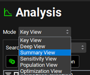
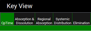
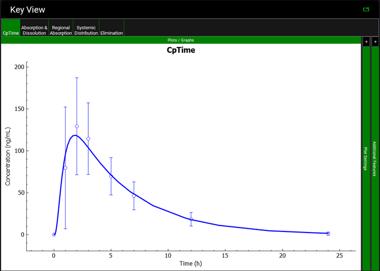
Switch the mode on the Analysis view back to Key View and click the words CpTime in the ribbon underneath the words Key View in the main panel.
The predicted plasma concentration (Cp-Time) curve appears on the picture as a blue line with the observed data points as empty circles with error bars.
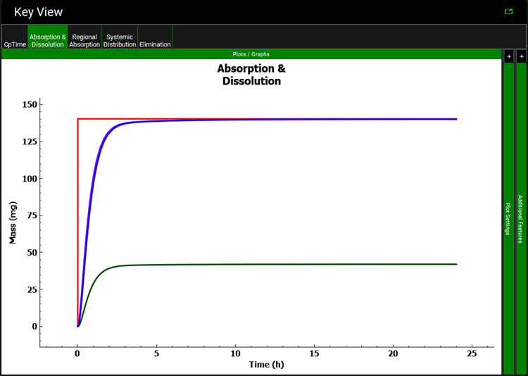
Clicking on Absorption & Dissolution displays the amounts dissolved (red curve), absorbed (purple curve, overlaid with the blue curve so not visible), in the hepatic portal vein (blue curve), and entering the systemic circulation (green curve).
Clicking on Regional Absorption displays a bar graph of the predicted amount absorbed in each Gut (ACAT) section.
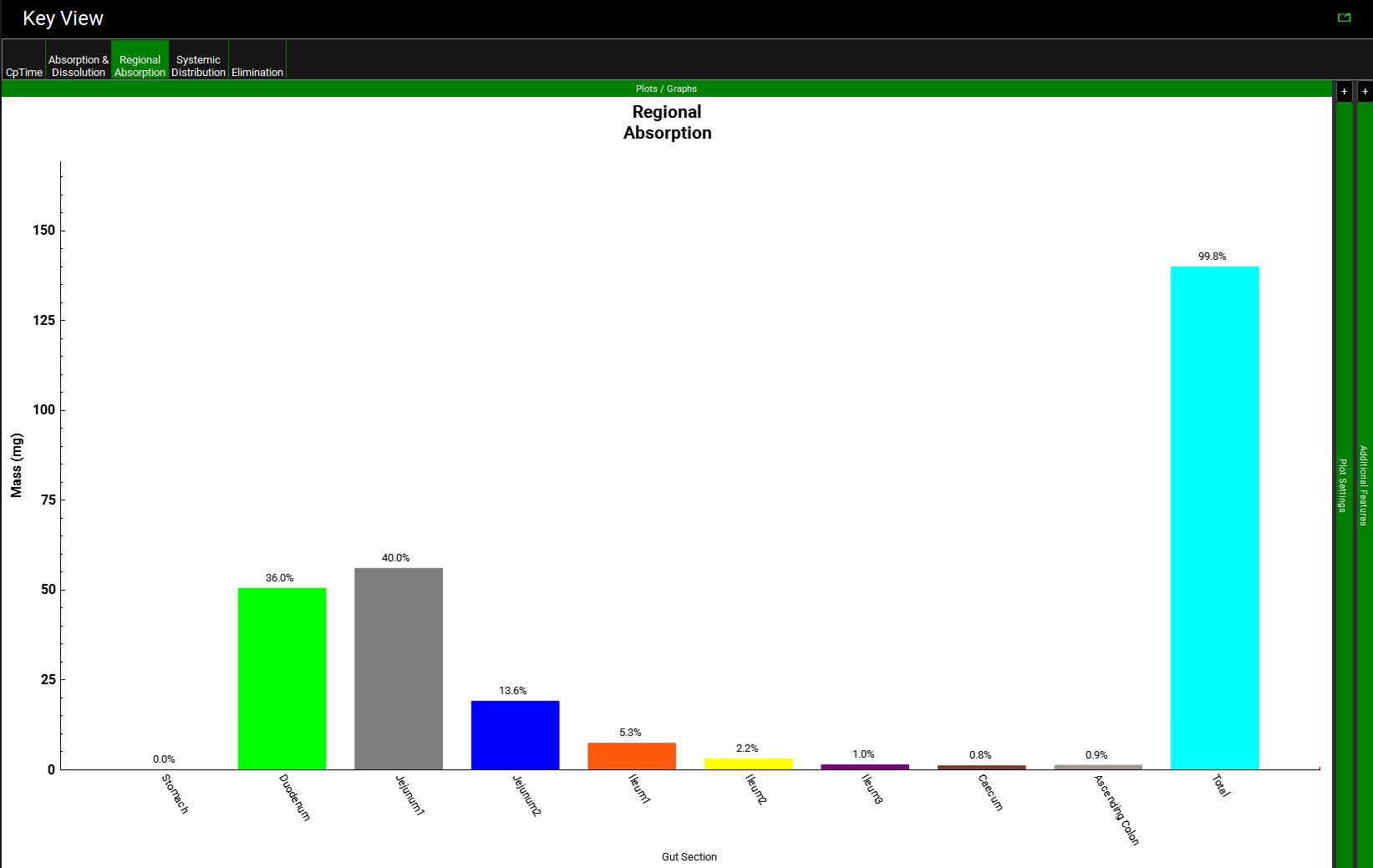

Because of the rounding of values for display purposes, the sum of the individual values might not equal the Total value in the Regional Absorption plot.
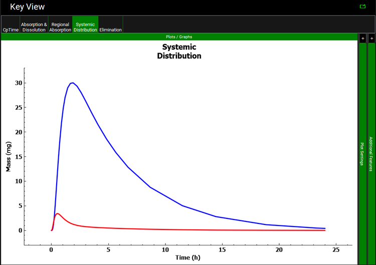
The Systemic Distribution Key View plot displays the amount in the systemic circulation (blue curve) and in the liver (red curve) as this simulation used a 1 compartment PK model.
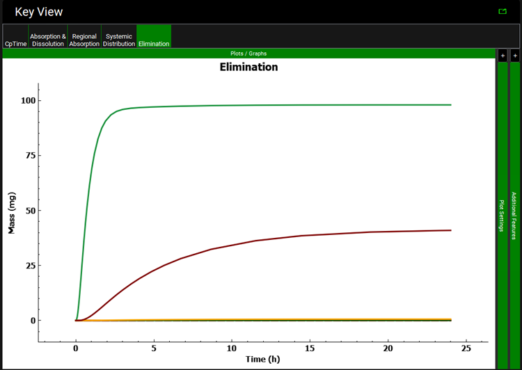
The Elimination Key View plot displays the amount eliminated via liver FPE (light green) and the amount eliminated through general clearance (brown). Other curves are available, namely the amount eliminated via gut metabolism and renal clearance and the dissolved and undissolved amount excreted from the GI tract, but these are negligible for this simulation.
We will now predict the Fa for each drug in the same way you did for Propranolol by doing a single run that includes all the compounds in this project.
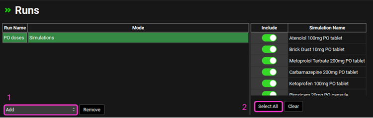
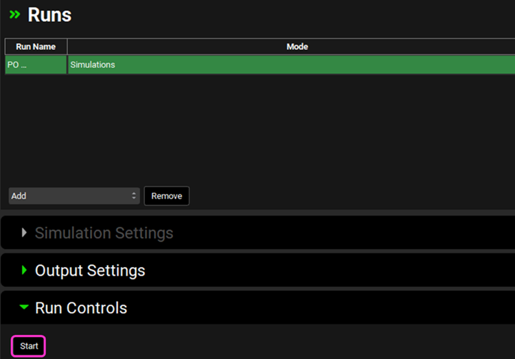
Navigate to the Runs view, click the Add button (which is at the bottom of the first column called Run Name), select Simulations and name your run (e.g., PO Simulations). Move to the right-hand side to the bottom of the Include column and click on Select All - all toggles next to the simulations will turn green. To deselect a simulation, click the toggle next to that specific Simulation Name – the toggle changes back to gray to indicate that the simulation is no longer selected.
Close the Output Settings panel and click start in the Run Controls panel.
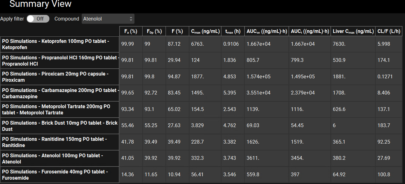
The Analysis view will automatically be activated when the Run has completed. Switch the Mode to Summary View, which enables you to compare the Fa for all compounds in this Project. For easier viewing, pop the table out into its own window using the green icon next to the Observed data on toggle.

To pop it back in, click the cross in the top right corner of the window.
Sort the compounds in order of Fa(%) by holding Alt and clicking on the column header. Observed data can be toggled on and off using the Observed data on toggle in the top right corner.