
GPX™ Run Modes Tutorial: Optimization
This tutorial explores the use of the optional Optimization module which can adjust a selected subset of a wide variety of model parameters in order to minimize an objective (error) function constructed from predicted and observed values.
In this tutorial, we will cover:
Optimization of the dose to achieve a specific Cmax
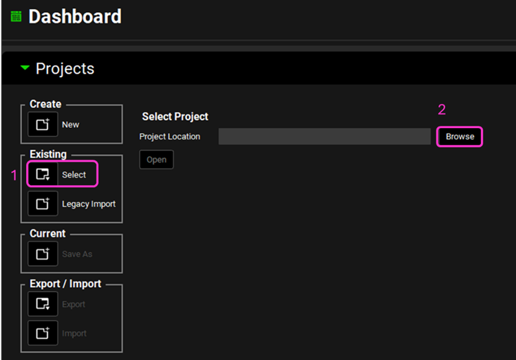
Open GPX™ and, in the Dashboard view, click on the icon next to Select to open an Existing project.
Click Browse and navigate to the C:\Users\<user>\AppData\Local\Simulations Plus, Inc\GastroPlus\10.2\Tutorials\GPX Library and select the project file GPX Library.gpproject by clicking on it and clicking Open.
Save a copy of the project by clicking on the icon next to Save As, entering “Optimization Tutorial Brick Dust” as the Project Name and click Browse to navigate to/add a folder to Save the project in. Click Save - you will see an information message in the Messages Center indicating that the project has been successfully copied. This message will disappear once you click 'Yes' on the pop-up window that also appears. Note that the name of the project visible in the top right corner of the interface is the one that has just been created.
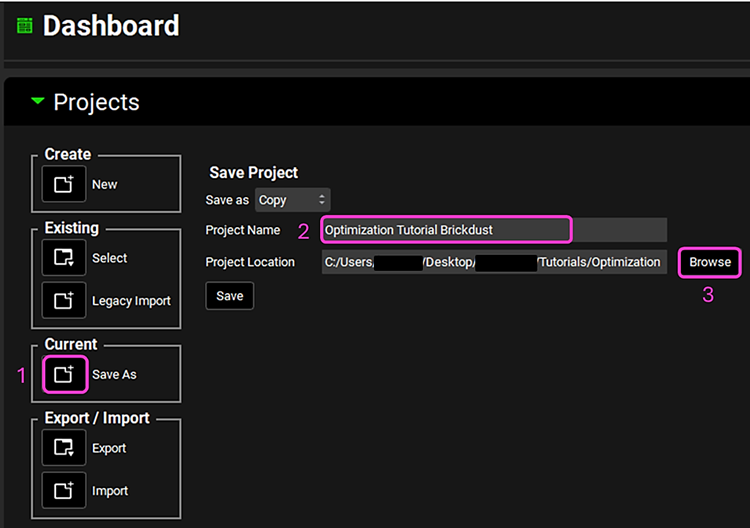
NB – numbers reflect the order of the steps in the screenshot, rather than corresponding to the steps in the tutorial.
Move through the views on the navigation pane from Compounds to Simulations, observing the information that has been entered in this project.
Move to the Simulations view, select the Brick Dust 10mg PO tablet as the simulation, click the Check Warnings button and then Run Simulation.
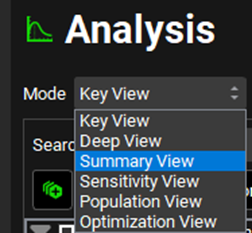
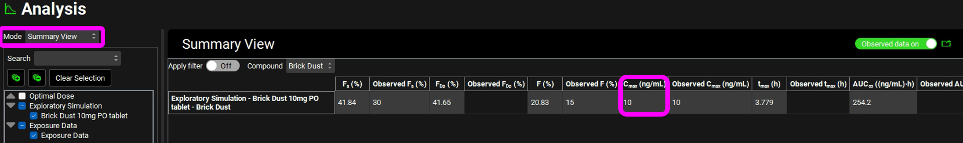
When the Simulation completes the program automatically switches to the Analysis View. Switch the Mode to Summary View and observe that the predicted Fa is approximately 55% and Cmax is approximately 3.8 ng/mL.
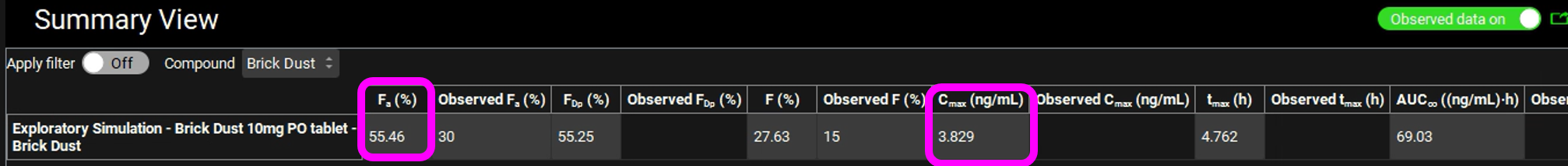
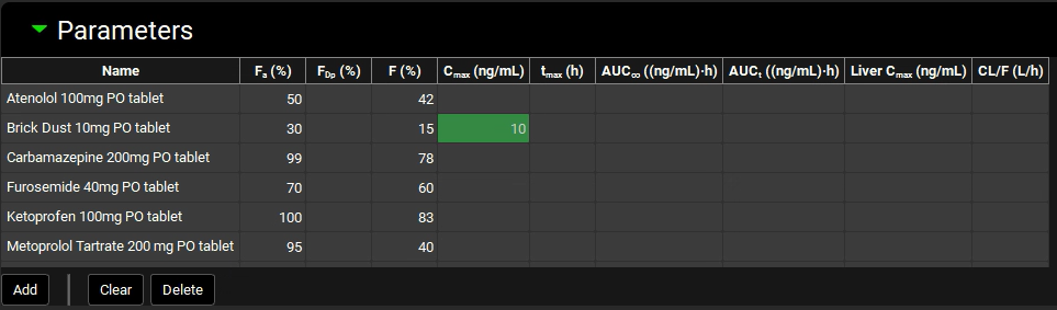
We are going to optimize the dose such that a Cmax of 10 ng/mL is obtained.
Navigate to the Observed Data view, minimize the Profiles panel (by clicking on the green arrow or double clicking on the Profiles panel header bar) and expand the Parameters panel. Enter 10 ng/mL as the observed Cmax for Brick Dust 10mg PO tablet by typing in the appropriate cell and hitting Enter.
Save the project by clicking on the Save button in the top right corner of the interface and clicking OK on the Save completed message.
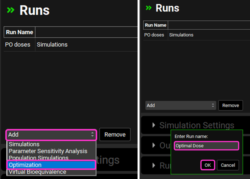
Navigate to the Runs view.
Click Add, select Optimization as the Run type and name it “Optimal Dose” before clicking OK.
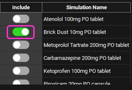
Select the Brick Dust 10mg PO tablet simulation from the list of Simulations on the right.
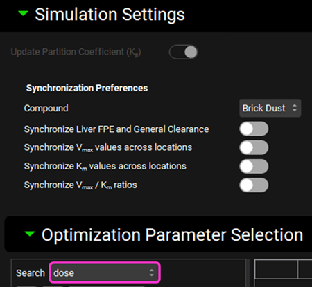
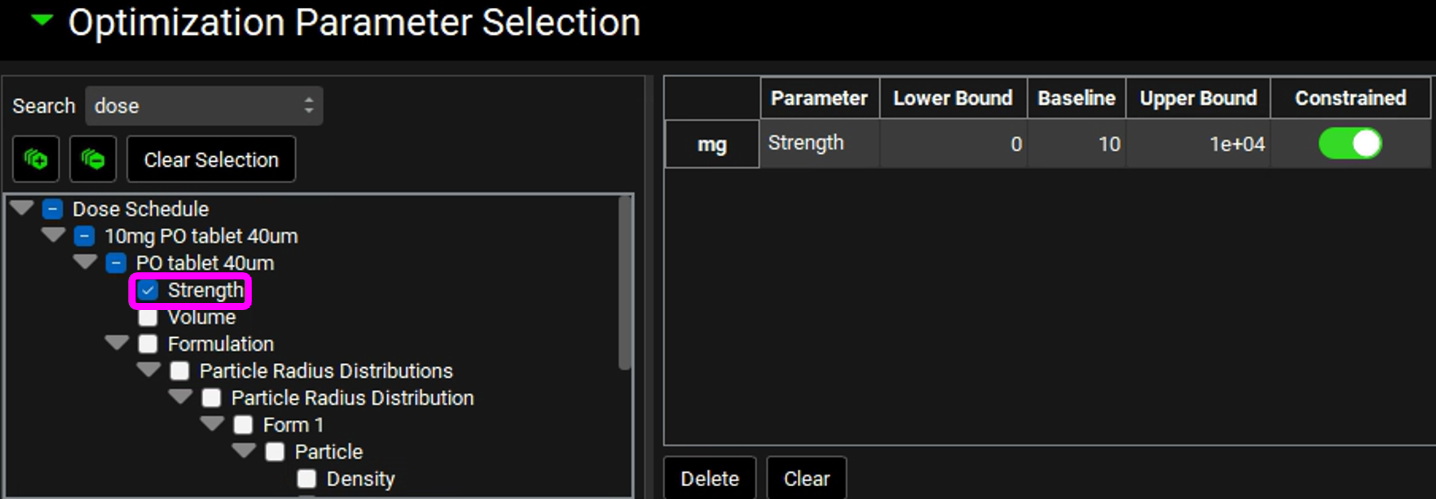
In the Simulation Settings panel, move to the Search box in the Optimization Parameter Selection sub-panel, type “dose” and hit return.
Check the box next to “Strength” under PO tablet 40µm in the Series List tree. This populates the table to the right of the tree with the selected parameter and enables the bounds to be set.
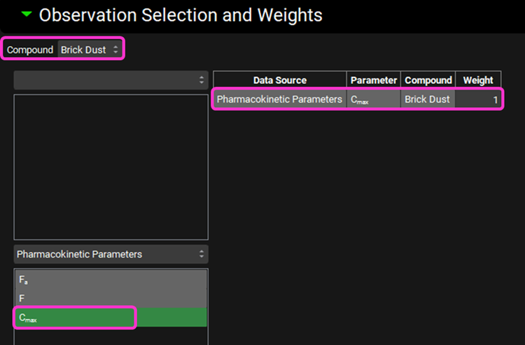
In the Observation Selection and Weights sub-panel below, click on Cmax in the Pharmacokinetic Parameters to select it. The parameter is added to the table on the right for the selected compound and the objective weight is automatically set to 1, which is correct for this example, but can be edited if required.
Save the project and click OK.
Scroll down to view the Run Controls panel and click Start to begin the optimization.
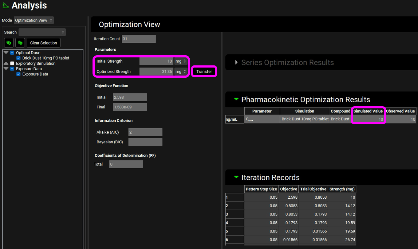
When the optimization completes the interface will automatically switch to the Analysis view using the Optimization View mode.
The Optimization View displays the initial dose as well as the optimized dose of 31.3mg. Next to the optimized value is a button labelled Transfer which enables the final value to be transferred to the appropriate input field. The Pharmacokinetics Optimization Results are also shown which confirms that the simulated Cmax achieved is 10 ng/mL.
Click Transfer to update the administered dose.
Note the message that appears in the Messages Center that confirms the update that has been made and highlights in which panel the change has been made. Click Done to clear the message.
In addition to the results displayed in the user interface, an excel file called ”optimization results” followed by the date and time in the title, optimization resultsDate Time.xlsx, is generated. This is found in the same folder as the project, in a subfolder named as per the run name. So, in this case, the subfolder would be called “Optimal Dose”. The worksheet Optimization Iterations shows the different doses that were simulated, and the final row will contain the final optimized value. Note that the units may differ from those used in the interface. The parameters chosen for optimization, along with the bounds, are displayed on the Optimization Parameters worksheet.

Note: the Optimization Summary worksheet will be blank for this example, it will be populated for optimizations run using an observed profile (see next example To calibrate an absorption model for a drug based on an observed Cp-Time profile).
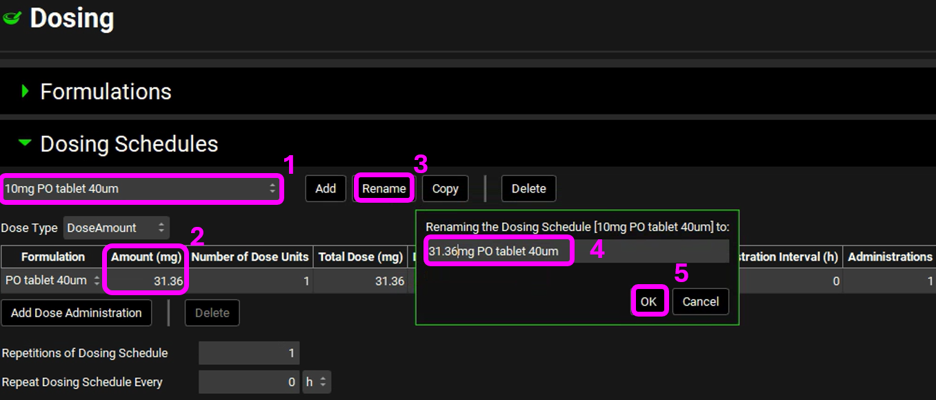
Navigate to the Dosing view and, if necessary, expand the Dosing Schedules panel. Select the 10mg PO tablet 40um Dosing Schedule from the drop-down menu and confirm that the Amount (mg) has been updated to 31.36mg. For completeness this can be renamed to reflect the dose administered by clicking on the Rename button and editing 10mg to 31.36mg before clicking OK.
Save the project and click OK.
Navigate to the Simulations view, Check Warnings and then Run Simulation.
When the simulation has completed, switch the Analysis view Mode to Summary View and confirm that the Cmax achieved is approximately 10 ng/mL.
To calibrate an absorption model for a drug based on an observed Cp-Time profile
Open GPX™ and, in the Dashboard view, click on the icon next to Select to open an Existing project.
Click Browse and navigate to the C:\Users\<user>\AppData\Local\Simulations Plus, Inc\GastroPlus\10.2\Tutorials\Optimization Project A and select the project file Optimization Project A.gpproject by clicking on it and clicking Open.
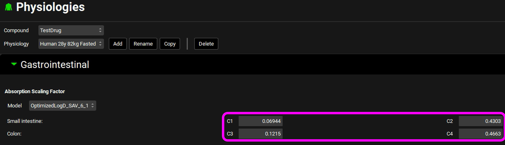
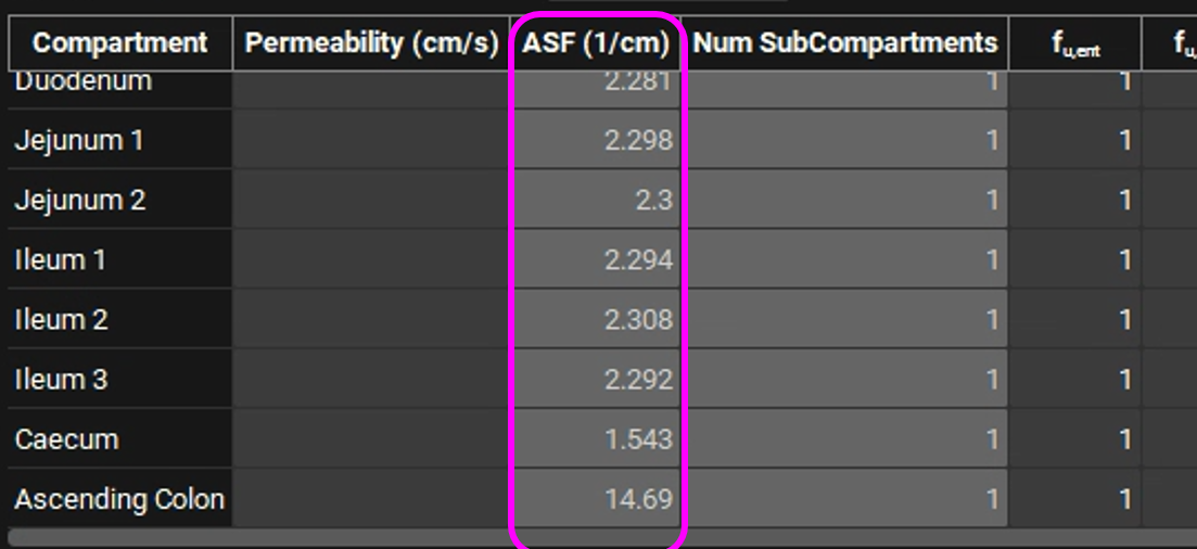
Move through the views on the navigation pane from Compounds to Simulations, observing the information that has been entered in this project. It contains one compound called TestDrug. Let us assume that the pharmacokinetic parameters are known (CL=1.0 L/h/kg, Vc = 1.0 L/kg) for this drug (found in the Pharmacokinetics view in the Compartmental panel) but not the Peff (found in the Compounds view in the Permeability panel) or the ASFs (which can be seen on the Gastrointestinal panel in the Physiologies view). The mean oral Cp-Time curve for this compound is available in the Observed Data view, Profiles panel.
Navigate to the Simulations view. Run the simulation “TestDrug 100mg PO Tablet”.
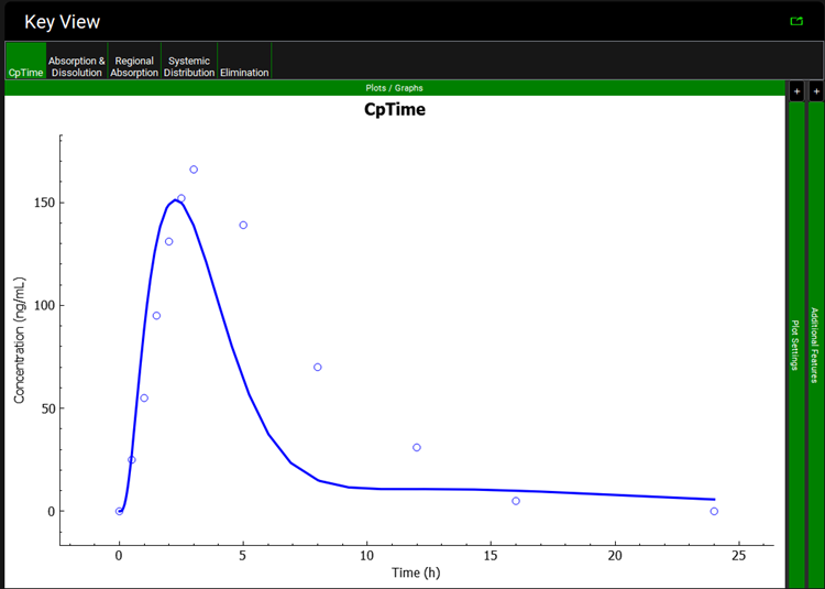
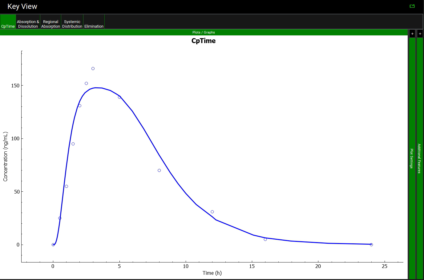
When the simulation completes the interface will automatically switch to the Analysis view. The Cp-Time Key View plot is displayed, and it can be seen that the simulated profile (indicated by the blue line) underpredicts the observed data (indicated by the blue points).
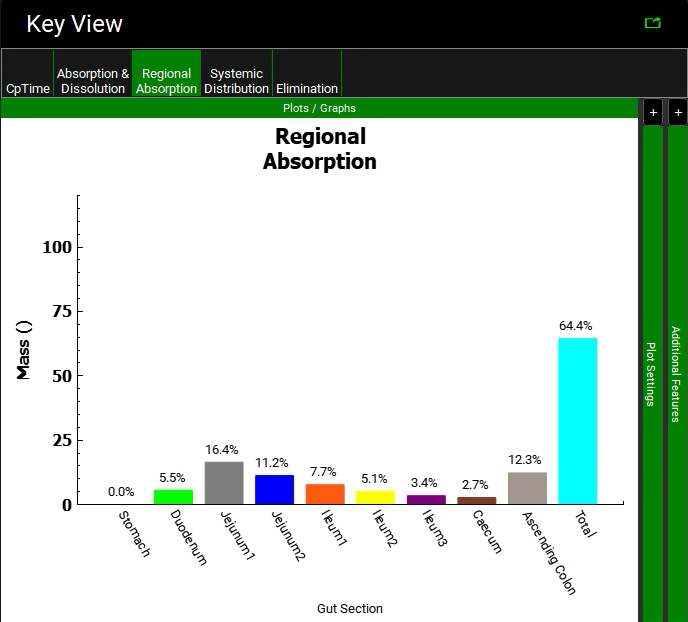
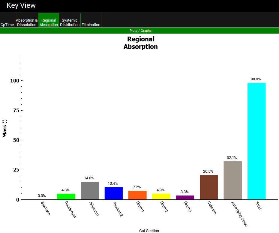
Click on the Regional Absorption plot in the Key View ribbon to see that 2.7% and 12.3% of the dose is absorbed in Caecum and Ascending colon and that total absorption is less than 100%.
Assuming all inputs other than the Peff are correct, the absorption model needs to be calibrated for this drug. Calibration of the absorption model consists of fitting the Peff and/or the ASFs to produce an absorption rate profile that will result in the observed Cp-Time curve. Since we do not know the Peff or the ASFs in this case, we will calibrate the absorption model by fitting the ASFs alone. With the logD models, the ASFs are calculated based on the absorption gradient coefficients C1-C4 seen on the Physiologies view in the Gastrointestinal panel.
Rather than optimizing the 8 individual ASF directly, one for each gastrointestinal compartment (except the Stomach), we will optimize the four gradient coefficients of the ASF model to calibrate an absorption model.
Save the project and click OK.
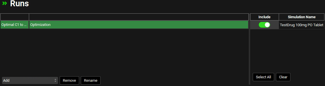
Navigate to the Runs view.
Click Add, select Optimization as the Run type and name it “Optimal C1 to C4” before clicking OK (or pressing Enter).
Select the TestDrug 100mg PO tablet simulation from the list of Simulations on the right.
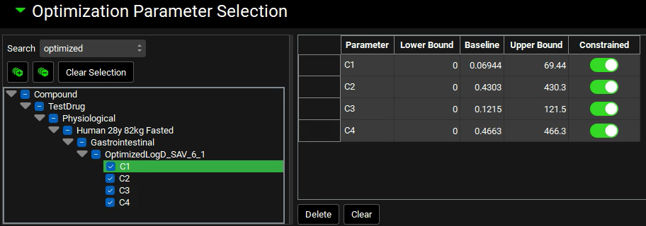
In the Simulation Settings panel, move to the Search box in the Optimization Parameter Selection sub-panel, type “Optimized” and hit return.
Check the boxes next to each of the “C1” to “C4” under OptimizedlogD_SAV_6_1 in the Series List tree. This populates the table to the right of the tree with the selected parameters and enables the default bounds to be adjusted, if required. For this example, we will use the defaults.
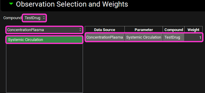
In the Observation Selection and Weights sub-panel below, ensure ConcentrationPlasma is selected and click on Systemic Circulation to select it. The parameter is added to the table on the right (for the selected compound only) and the objective weight is automatically set to 1, which is correct for this example, but can be edited if required. This ensures that we are optimizing against the observed Cp-Time profile.
Scroll down within the Observation Selection and Weights sub-panel and ensure that the Objective Weighting is set to 1/y^2.

Save the project and click OK.
Scroll down to view the Run Controls panel and click Start to begin the optimization.
Notice that the Rsq: TestDrug – Systemic Circulation of the fit is ~ 0.6 at the beginning of the optimization and steadily increases as the optimization proceeds. You can stop the optimization by clicking on the Stop button when a desired accuracy (e.g. Rsq > 0.9) has been achieved instead of waiting for the optimizer to end the process.
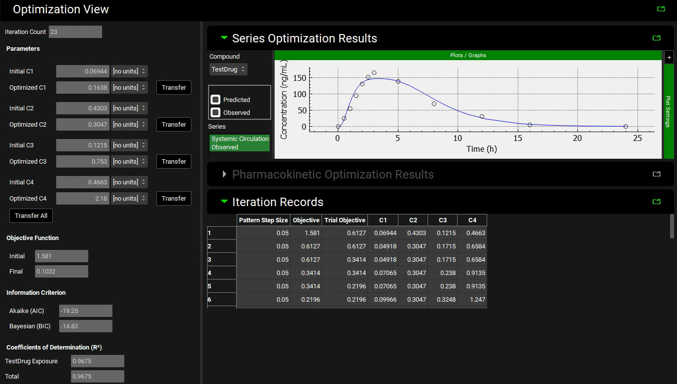
When the optimization completes the interface will automatically switch to the Analysis view in the Optimization View Mode.
The Optimization View displays the initial parameter values as well as the optimized values. Next to each of the optimized values is a button labelled Transfer which enables the final value to be transferred to the appropriate input field. To transfer all of the optimized values with one click, a Transfer All button is at the bottom of the list of parameters. The Series Optimization Results are also shown which allows the observed Cp-Time profile to be compared against the profile simulated using the optimized parameters. Some statistical measures, for example the R2 and Akaike Criterion, are also displayed.
Click Transfer All button to update C1 to C4. Note the messages that appear in the Messages Center that confirm the update has been made for each parameter and lists which panel the change has been made in. Click Done to clear each message.
The optimization results are captured in an excel file, optimization results.xlsx, stored in the same folder as the project, in a subfolder named as per the name of the run (“Optimal C1 to C4” for this example). The worksheet Optimization Summary contains the final predicted concentrations, together with the observed plasma concentrations that were used for optimization and the resulting residuals. The worksheet Optimization Iterations displays the different values that were used during the optimization and the final row contains the final optimized values. The parameters chosen for optimization, along with the bounds, are captured on the Optimization Parameters worksheet.
Navigate to the Physiologies view and expand the Gastrointestinal panel. Examine the new parameter values. The change in C1 to C4 has caused a change in the ASFs - with the optimized absorption gradient coefficients, the Caecum and Ascending Colon ASFs are both significantly higher than predicted by the default Opt logD Model SA/V 6.1. We have now obtained an ACAT absorption model calibrated for this particular drug. If the Cp-Time curve from more than one dose is available, the model can be optimized over all the doses, and a more accurate model will be obtained.
Save the project and click OK.
Navigate to the Simulations view and rerun the simulation using the newly optimized absorption gradient coefficients. Because the values have been updated in the original physiology, no changes need to be made to the Simulation Settings.
A single simulation has now been run and when it completes it will automatically switch to the Analysis view, displaying the last Key View plot viewed. Navigate to the Cp-Time Key View plot if necessary. It can be seen that the simulated profile predicts the observed data.
Click on the Regional Absorption plot in the Key View ribbon to see that the Caecum and Ascending Colon absorption fractions have increased to approximately 21% and 32% of the dose for the optimized logD model. The total absorption is close to 100%. Your result may be different depending on when you stopped the optimization and the solution the optimizer found.
Care should be taken in running an optimization to ensure that the correct parameters are chosen for optimization such that full use is made of the experimental data and covariant variables are avoided. Optimization is a very powerful tool, but it must be used correctly to get the best results.