
GPX™ Run Modes Tutorial: PSA Using GPX™ Library Project
Input values for some of the physicochemical properties of a compound are often estimates that are obtained by different methods, such as from an in silico prediction or from in vitro testing. Frequently, the values that are obtained by these methods do not correlate exactly with their in vivo values. If a compound has a poor predicted fraction absorbed (Fa) or bioavailability (F), then it is beneficial to know the factors that are limiting the absorption or bioavailability. Parameter Sensitivity Analysis (PSA) assesses the effect of varying the value for a single parameter at a time while holding all other parameters constant at their baseline values. The output from this analysis can help in identifying the factors that limit the Fa or F for the compound of interest and methods devised to overcome these limitations, such as excipients, salt formulations, co-solvents, permeability enhancers etc.
This tutorial explores the use of a sequential PSA to determine the two primary parameters that limit the solubility of “Brick Dust” (a fictional compound with properties similar to fosinopril) and then a cross PSA to determine the impact of those two parameters in combination.
This tutorial has two parts:
PART 1 – Sequential PSA
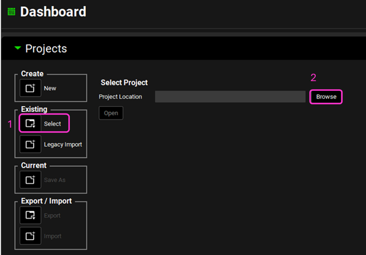
Open GPX™ and, in the Dashboard view, click on the icon next to Select to open an Existing project.
Click Browse and navigate to the C:\Users\<user>\AppData\Local\Simulations Plus, Inc\GastroPlus\10.2\Tutorials\GPX Library folder and select the project file GPX Library.gpproject by clicking on it and clicking Open.
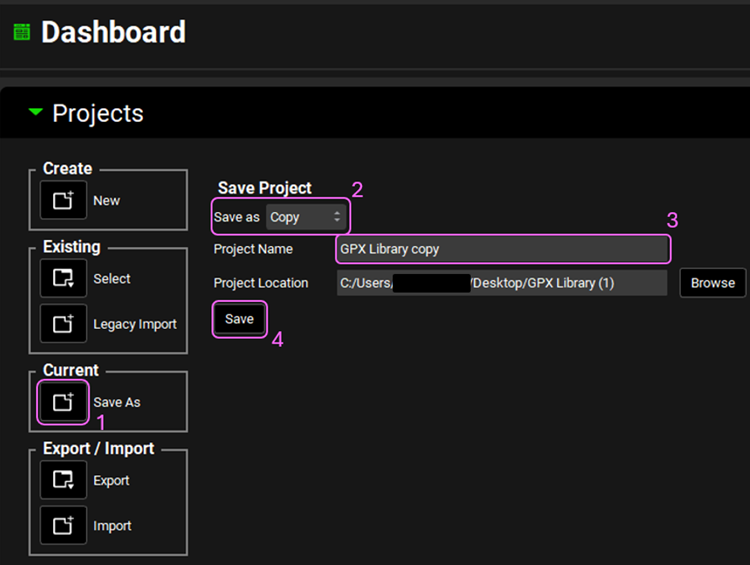
Now we will save a copy of the Library project to keep the original project unaltered. In the Dashboard view, click on the icon next to Save As under the Current frame. From the Save as drop-down, select Copy. Type GPX Library copy as the Project name and click Browse to navigate to/add a folder to Save the project in. Click Save - you will see an information message in the Messages Center indicating that the project has been successfully copied. This message will disappear once you click 'Yes' on the pop-up window that also appears.
Note that the project name is now GPX Library copy on the top right-hand side.

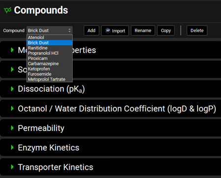
Navigate to the Compounds view. From the Compound drop-down, select Brick Dust. Open the panels by double clicking on the panel header or on the green arrow and observe the data that has been entered for it.
Navigate to the Simulations view and select Brick Dust 10mg PO tablet simulation. The Drug Administration panel displays the following information for the Brick Dust compound: Compound (name), Dose Schedule, Dose Number, Absorption Number, and Dissolution Number.
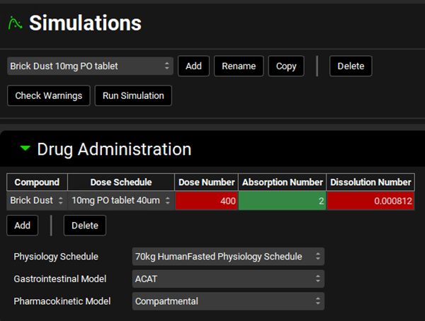
Note that the Dose Number and Dissolution Number are red while the Absorption Number is green, suggesting that solubility might be a limiting factor for absorption.
Click on Check Warnings then Run Simulation buttons. After the simulation is completed, the Analysis view opens. By default, it opens in Key View and the Cp-Time plot is displayed.
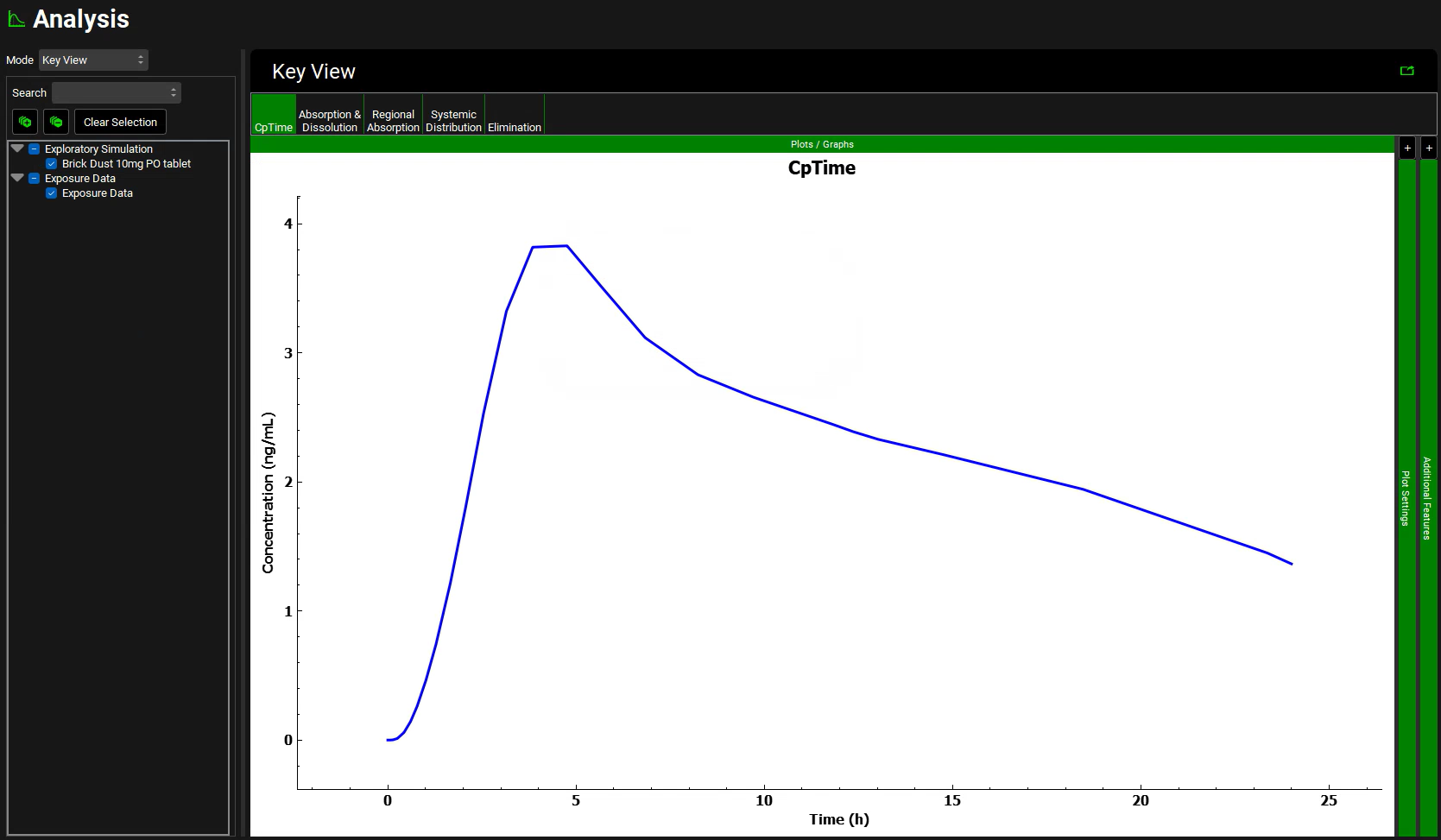
The simulated curve can be smoothed by decreasing the Output Frequency in the Configuration panel within the Simulations view. This causes GastroPlus® to calculate time steps more frequently, resulting in a smoother curve.
Click on the Absorption & Dissolution plot in the Key View ribbon. By default, all available Mass vs. Time curves for the Absorption & Dissolution plot are displayed.
Open the Plot Settings panel by clicking on the “+” at the top of the bar to display the legend. Uncheck the Systemic Circulation Mass Entered curve and the Total Portal vein curve. Hover over the legend to see the whole legend name.
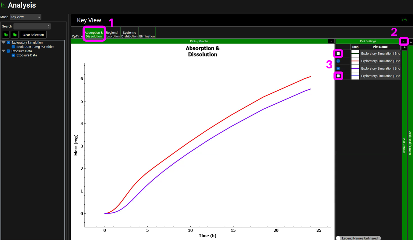
Because some of these curves are only slightly divergent from other curves, and therefore, not easily distinguishable on the plot, the default plot is not shown here.
The two remaining curves on the plot are the curves for Total Amount (of Brick Dust) Dissolved (the red curve) and Total Amount (of Brick Dust) Absorbed (the purple curve). The plot clearly shows that the Brick Dust dose was not completely dissolved in 24 hours (red curve) and that the absorption curve (purple curve) diverges only slightly from the dissolution curve, which indicates the absorption of Brick Dust is primarily solubility-limited.
On the Mode drop-down list, select Summary View.
Note that the predicted Fa(%) is just over 55%, which means that only about 55% of the compound is absorbed in the GI tract in 24 hours.
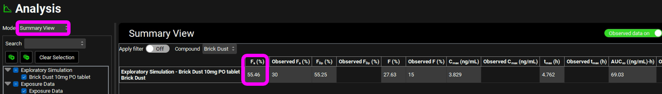
A Parameter Sensitivity Analysis can help to determine the degree to which permeability, solubility, and dissolution limit the absorption of this drug, and therefore how we can enhance the Fa.
Navigate to the Runs view and select Parameter Sensitivity Analysis from the Add drop-down.
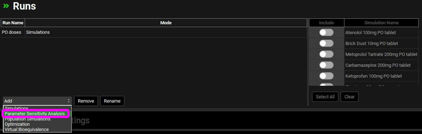
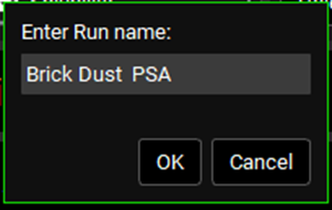
The Enter Run name dialog box will appear. Type Brick Dust PSA and click OK or press Enter.
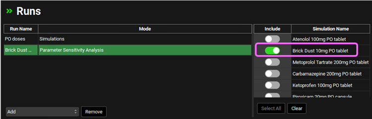
The run is added to the Runs list and the list of available simulations to be included in the run will be enabled. Click on the Include toggle next to the Brick Drug 10mg PO tablet Simulation Name.
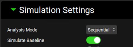
Expand the Simulations Settings panel. Leave the Analysis Mode as Sequential and leave the Simulate Baseline toggle on.
Scroll down to the parameters selection list from which you can select which parameters you wish to vary for the PSA.
In this tutorial, select Median Particle Size, Solubility, Tablet Strength, and Permeability.
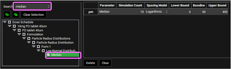
Type “median” in the Search box and press Enter. Select the box next to Median in the hierarchy tree.
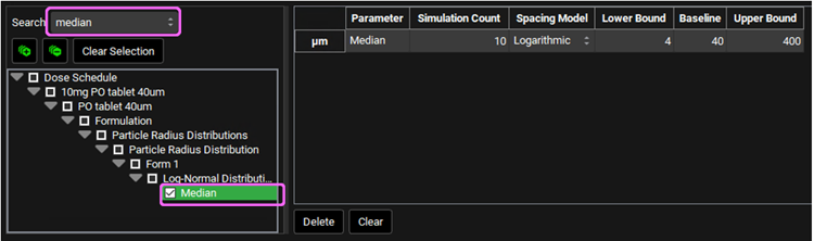
As you select an input parameter in the Simulation Parameters list, a Simulation Parameters table opens to the right of the list, and it is automatically populated with the Baseline values for each of the selected parameters. The Lower Bound and Upper Bound values are also displayed for each Baseline value.
If you wish to change the Simulation Count number, the Spacing Model, or the values for the Bounds and/ or Baseline, you can do so directly on the table.
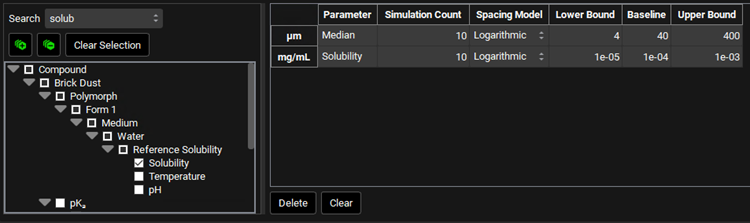
Type “solub” in the Search box and press Enter. Select the box next to Solubility in the hierarchy tree.

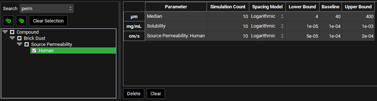
Type “perm” in the Search box and press Enter. Select the box next to Human in the hierarchy tree.
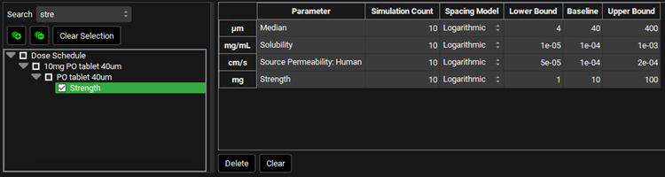
Type “stre” in the Search box and press Enter. Select the box next to Strength in the hierarchy tree.
You have two options for locating and selecting the necessary simulation parameters. You can manually expand the list, or you can use the Search feature.
Scroll down to the Run Controls panel and click on Start.
The Analysis view will automatically appear when the Run is completed.
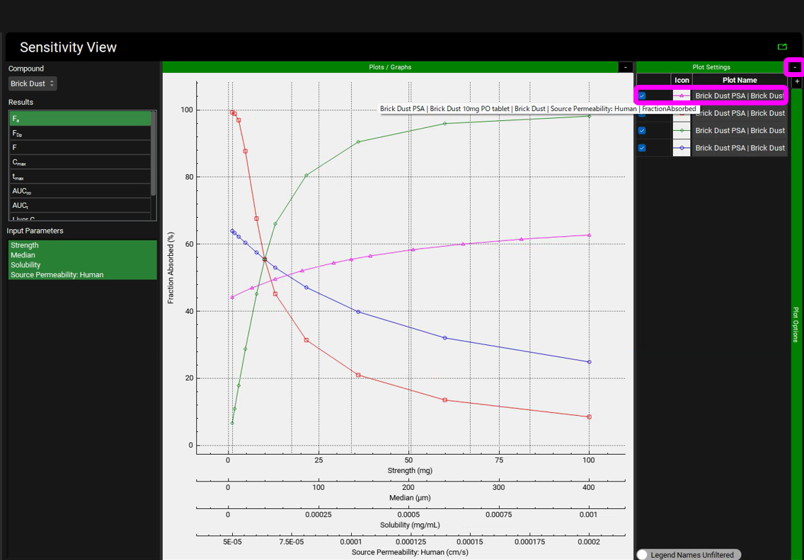
The Sensitivity View Mode is automatically selected for a PSA run. On the left side of the blank Plot, you will find the Compounds drop-down list, which is a list of all the compounds that are in the simulation used for the PSA (In this tutorial, we had a single compound, Brick Dust), a Results list from which you can select which parameter you wish to assess (such as Fa) and an Input Parameters list, which is a list of all the input parameters selected for the PSA run.
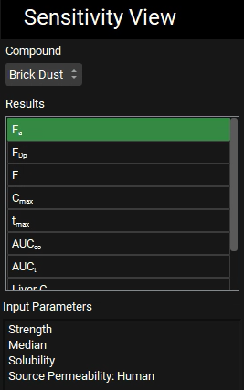
Select Fa from the Results list and select all parameters from the Input Parameters list.
To select multiple non-contiguous Input Parameters, hold down CTRL and Click on the input parameters you wish to select. To select all Input Parameters in a single step, use the Window [CTRL]+A keyboard shortcut. You can also click on the first parameter and drag the mouse down.
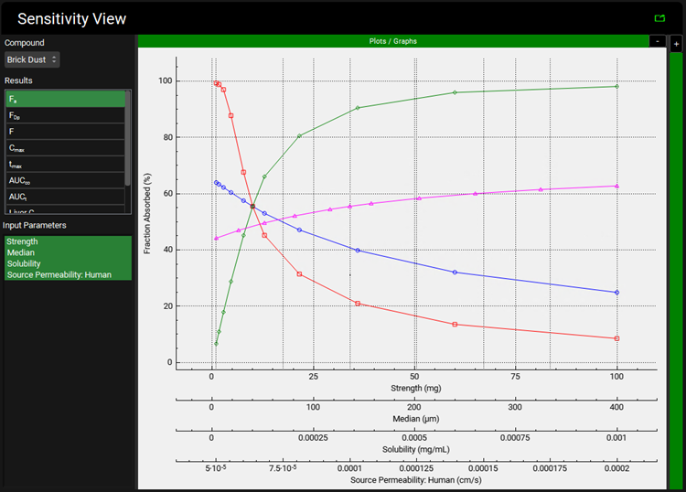
The output indicates that – within the range of values tested - the percent absorbed is extremely sensitive to solubility (green curve) and particle size (red curve), while it is less sensitive to permeability or dose. Absorption of Brick Dust appears to be primarily limited by solubility and dissolution rate (particle size).
For you to identify which curve is which, expand the plot legends by clicking on the “+” sign on the top right-hand side of the plot. Hover over the curves to display the curve’s full name.
On the left-hand side there is a list of all simulations run during the PSA (named with each parameter value that was varied while holding all other parameters constant at their baseline values).
Switch the Mode to Key View and select the Cp-Time plot if it is not already selected.
The Cp-Time profile for each simulation is plotted. Click across the Key View ribbon to see the other plots (they will be very busy since all the curves for each simulation are plotted).
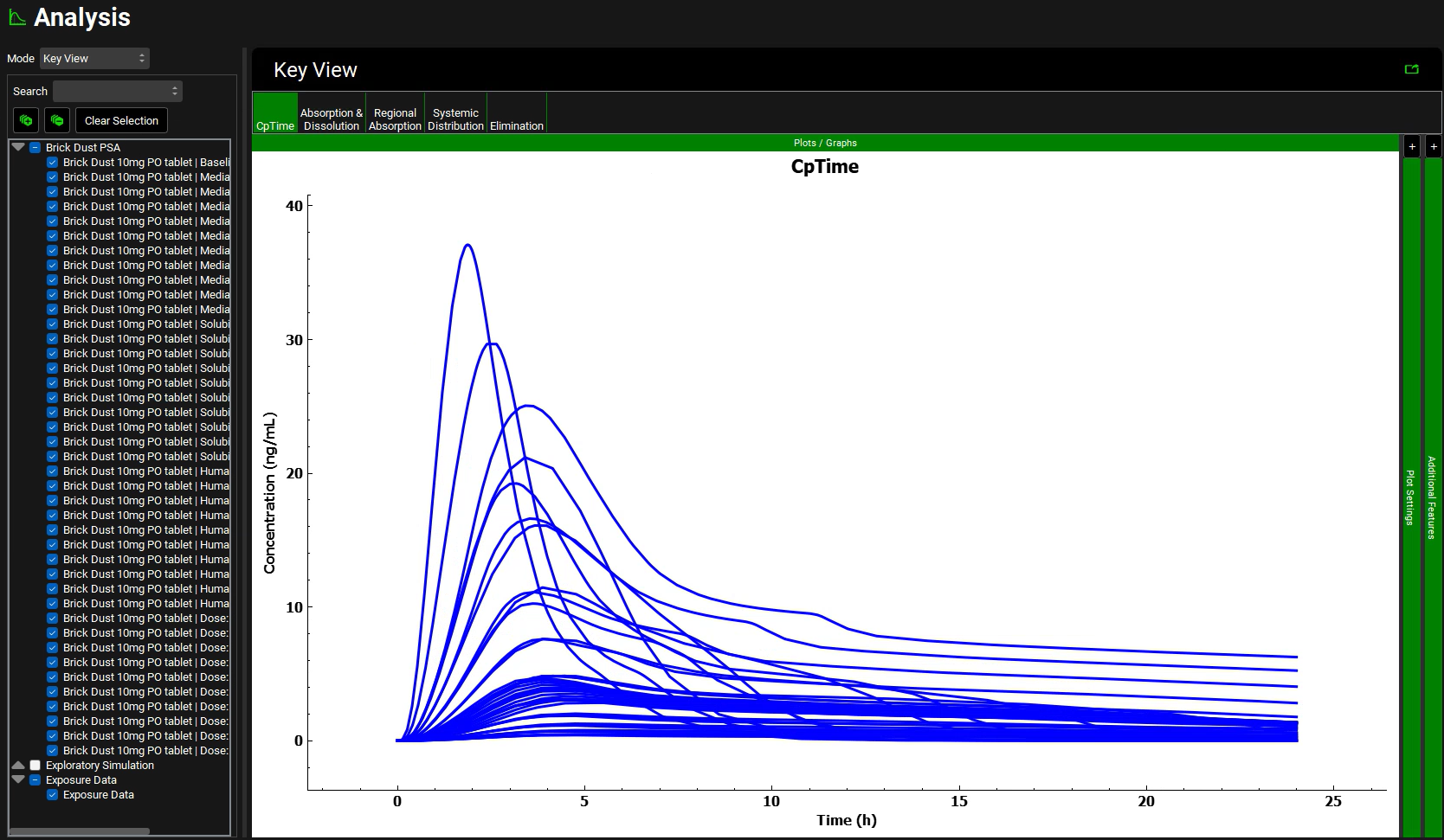
While on the Cp-Time plot expand the Plot Settings to see the legend. Click on the curve with the highest Cmax on the graph. The legend for that curve will be highlighted, hover over the highlighted legend to see the full name with the parameter and the parameter value.
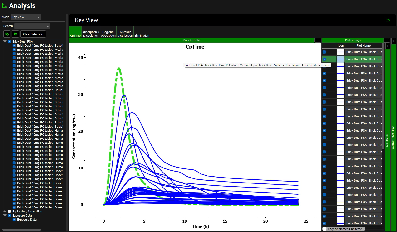
On the simulation list located left of the Key View panel, unselect all the curves by clicking on the box next to Brick Dust PSA twice. Once the selection has been cleared, select the simulation that had the highest Cmax (Median 4um). You may need to drag the simulation list panel to the right to be able to see the full simulation name.
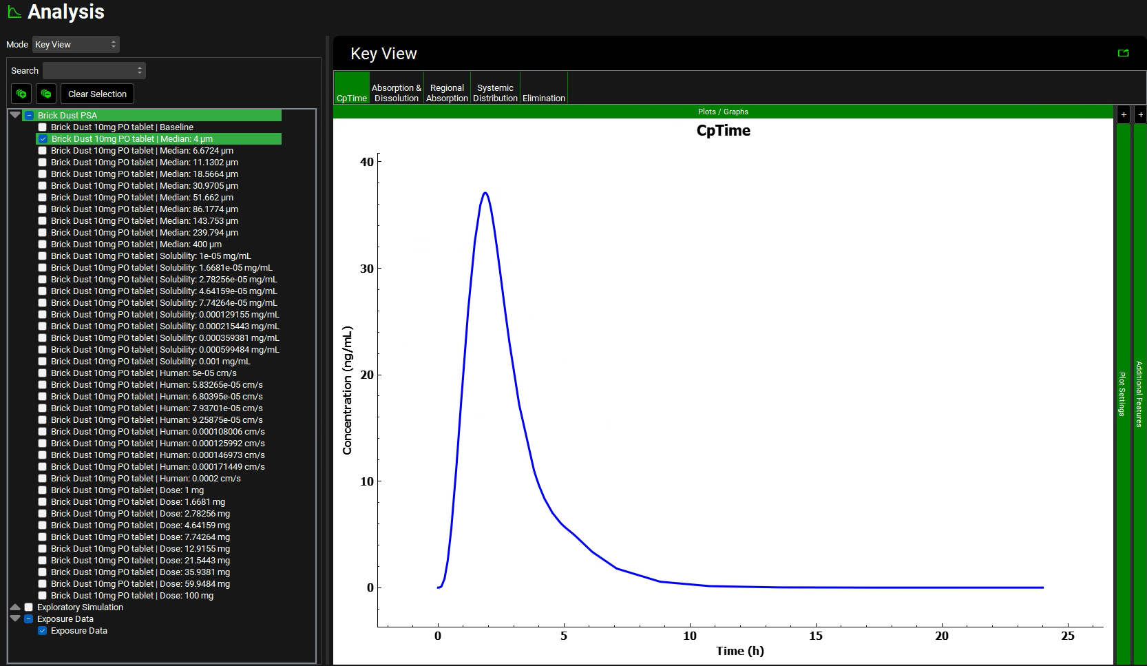
Now each plot in the Key View and Deep View will reflect only that simulation. Click across the plots in the ribbon and analyze the results. Return to the Cp-Time plot when finished.
Click on the check box next to Brick Dust PSA again to reselect all simulations.
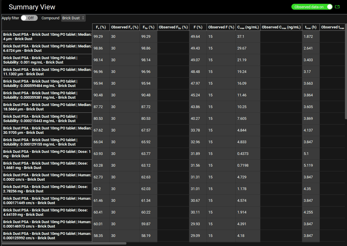
Switch the Mode to Summary View, which enables you to compare the Fa, FDp, F, Cmax, Tmax, AUC, Liver Cmax and CL/F for each subject in this run. Clicking on the column header while holding down Alt on your keyboard enables the simulations to be sorted in order of the values in that column.
PART 2 – Cross PSA
The previous example revealed that the absorption of the Brick Dust is primarily limited by solubility and dissolution. In this example we will examine a combined effect of these two processes.
Be sure that you have run Part 1 above before continuing.
Navigate to the Runs view and select Parameter Sensitivity Analysis from the Add drop-down.
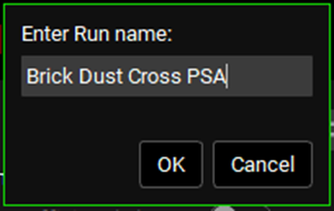
The Enter Run name dialog box will appear. Type Brick Dust Cross PSA and click OK or press Enter.
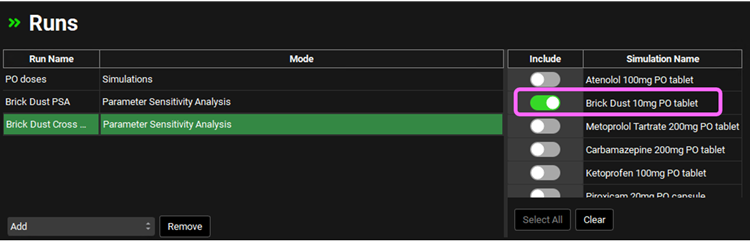
The run is added in the Runs list and the list of available simulations to be included in the run will be enabled. Click on the Include toggle next to the Brick Drug 10mg PO tablet Simulation Name.
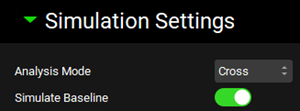
Expand the Simulations Settings panel. Switch the Analysis Mode to Cross and leave the Simulate Baseline toggle on.
Scroll down to the parameters selection list from which you can select which parameters you wish to vary for the PSA.
In this tutorial we will select Median Particle Size and Solubility.
Type “median” in the Search box and press Enter. Select the box next to Median in the hierarchy tree.
As you select an input parameter in the Simulation Parameters list, a Simulation Parameters table opens to the right of the list, and it is automatically populated with the Baseline values for each of the selected parameters. The Lower Bound and Upper Bound values are also displayed for each Baseline value.
If you wish to change the Simulation Count number, the Spacing Model, or the values for the Bounds and/ or Baseline, you can do so directly in the table.
Type “solub” in the Search box and press Enter. Select the box next to Solubility in the hierarchy tree.
You have two options for locating and selecting the necessary simulation parameters. You can manually expand the list, or you can use the Search feature.
Scroll down to the Run Controls panel and click on Start.
The Analysis view will automatically appear when the Run is completed.
Select Fa from the Results list and Solubility for the x-axis in the Input Parameters. Leave the y-axis as Median.
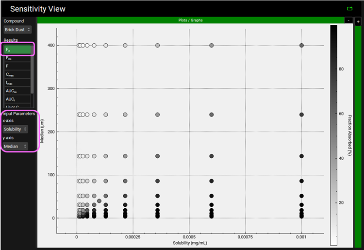
The gray scale dots plot will be displayed. On the scale on the right-hand side of the graph, you can see that the lighter the dot, the lower the Fraction Absorbed will be. Conversely, the darker the dot, the higher the Fraction Absorbed will be.
Hover over any point to view the Particle size, Solubility values combination that yielded that Fraction Absorbed.
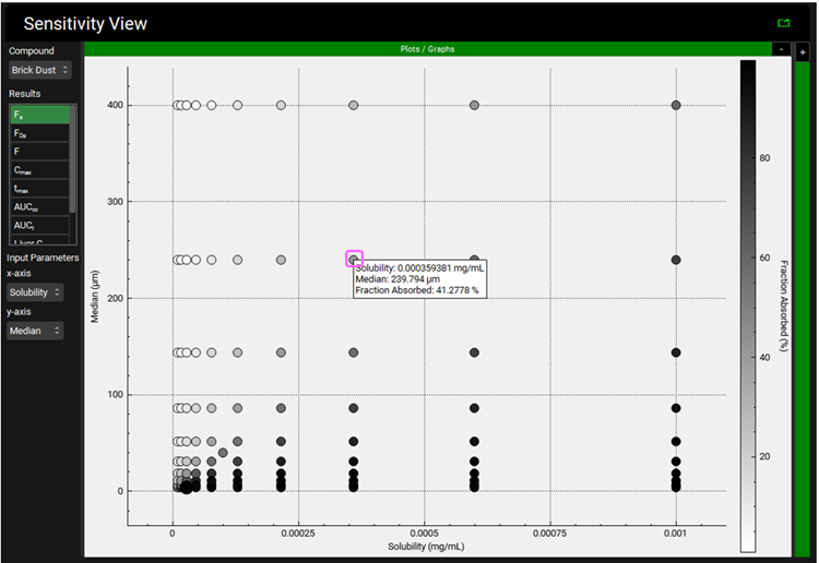
As shown in the screenshot, a solubility of ~3.6e-4 mg/mL and a Median particle size of ~240um would yield in a Fraction Absorbed of ~41.28%.
On the left-hand side of the Analysis view there is a list of all simulations run during the PSA (for each parameters value combination).
If you wish to do more in-depth analysis of any of these simulations, you can switch the Mode to Key View and Deep View and perform the desired assessments.