Tutorial: IVIVCPlus™ Module

IVIVCPlus™- In Vitro - In Vivo Correlation Module

IVIVCPlus™ includes numerical deconvolution, the traditional Wagner-Nelson and Loo-Riegelman deconvolution methods, as well as a state-of-the-art mechanistic deconvolution and one step correlation using the full GastroPlus® ACAT model for an oral dosage form. Mechanistic deconvolution can accommodate any combination of nonlinearities and complexities in the behavior of a drug. Numerical deconvolution and traditional methods are easy-to-use but are severely constrained by the simplifying assumptions that are necessary when using these approaches. Nonetheless, for some compounds, they are adequate. IVIVCPlus™ provides all of these recognized methods to give you a choice of how you want to perform your in vitro - in vivo correlations.

In this tutorial we will cover the following topics:

• Example 1: Loo-Riegelman (2-compartment model)

• Example 2: Numerical Deconvolution

• Example 3: Wagner-Nelson (1-compartment model)

• Example 4: Mechanistic (two-steps)

• Example 5: Multiple Subjects

• Example 6: Saving correlations and using them to generate an in vivo dissolution profile

Loo-Riegelman (2-compartment model)

This example illustrates the use of the Loo-Riegelman deconvolution method with a polynomial correlation function to generate an IVIVC with two different controlled release formulations of metoprolol. The resulting deconvolution is then used to predict the same two formulations as well as a third formulation.

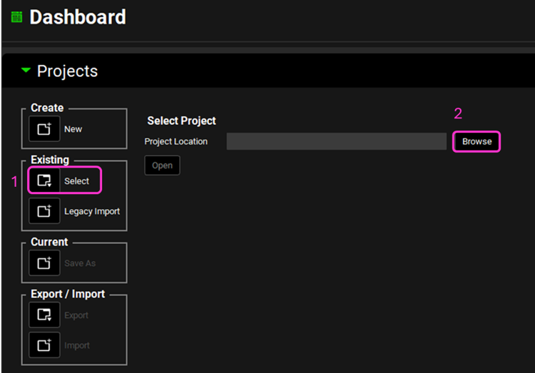
1. Open GPX™ and, in the Dashboard view, click on the icon next to Select to open an Existing project.

2. Click Browse and navigate to the C:\Users\<user>\AppData\Local\Simulations Plus, Inc\GastroPlus\10.2\Tutorials\Metoprolol-IVIVC folder and select the project file Metoprolol.gpproject by clicking on it and clicking Open.

3. Move through the views on the navigation pane from Observed Data to Simulations, observing the information that has been entered in this project.

4. In this project there is one compound (Metoprolol), one physiology (Human 30YO 66kg) and four different formulations (Fast CR Tablet, Moderate CR Tablet, Slow CR Tablet and New Form CR Tablet) with their respective Dosing Schedules.

In the Observed Data view, you will notice that there are both Exposure Data and In Vitro Dissolution Release for the Fast, Moderate and Slow formulations, while the New Form formulation only has In Vitro Dissolution Release data.

In the IVIVCPlus™ module, only assets that have both Exposure Data and In Vitro Dissolution Release data can be used for forming correlations. Assets with only In Vitro Dissolution Release data can be used for convolution to predict the likely C_p-Time profiles before dosing in subjects.

5. Navigate to the Pharmacokinetics view and note how there are two pharmacokinetic models linked to the Metoprolol compound: One compartment and Two compartments.

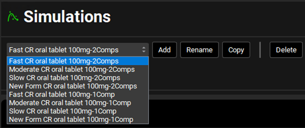
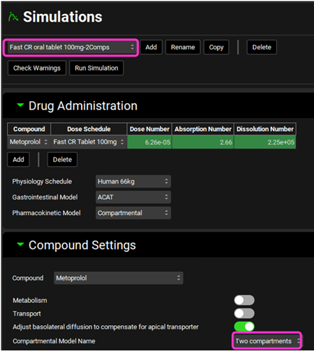
6. Navigate to the Simulations view. Click on the Simulations drop-down to see the simulations in this project. Note how there are two simulations for each formulation: one linked to the One compartment PK model (simulation name with “1Comp” ending) and another with the two Compartments PK model (simulation name with “2Comps” ending).

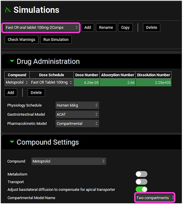
7. Select any of the “2Comps” simulations and expand the Compound Settings panel. Note that the Compartmental Model Name linked to it is “Two Compartments”. In this tutorial we will be using the “2Comps” simulations as the Base Simulation in IVIVCPlus™ (explained in more detail in later steps) since we are using the Loo-Riegelman2 deconvolution method.

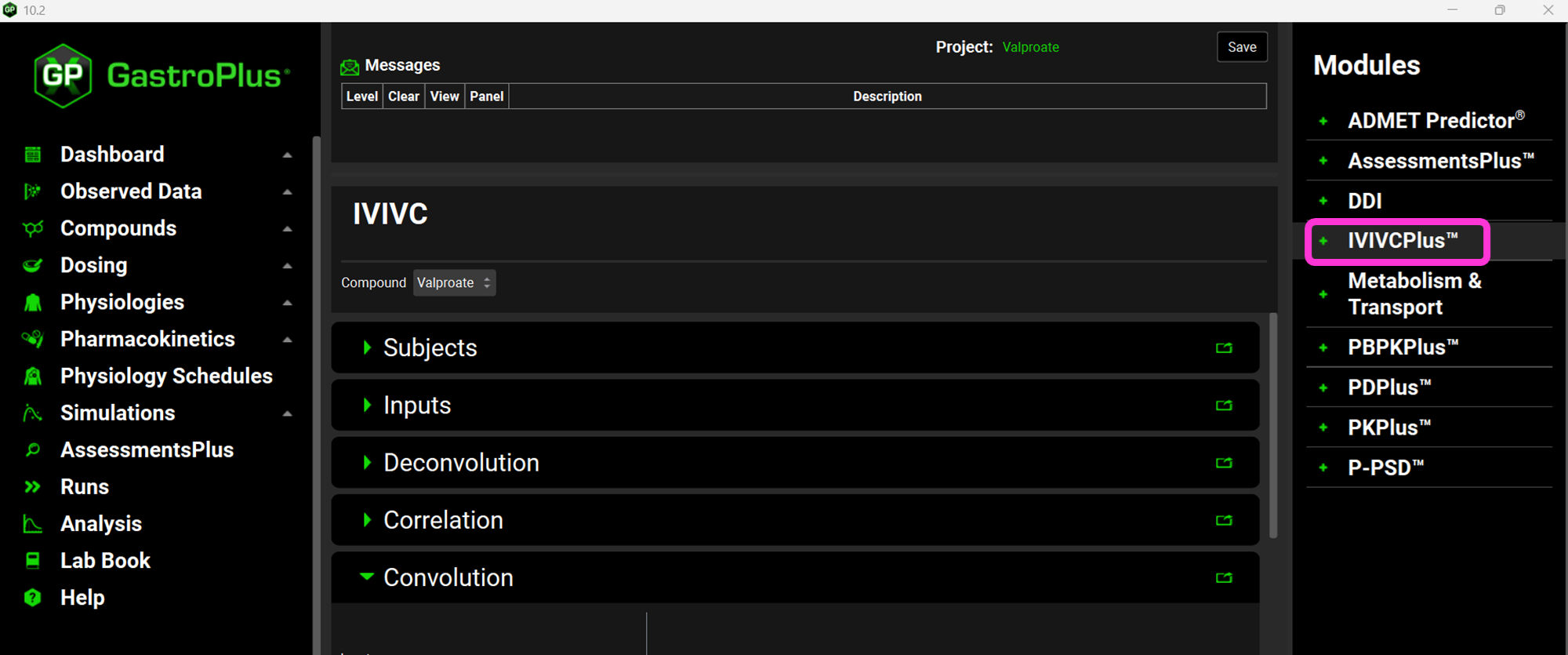
8. Click on IVIVCPlus™ in the Modules pane located on the right-hand side of the interface. The IVIVCPlus™ Module contains five panels: Subjects, Inputs, Deconvolution, Correlation and Convolution.

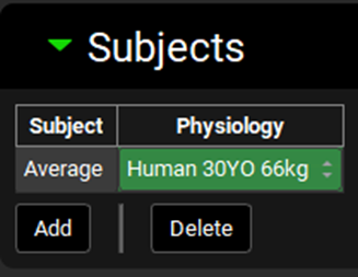
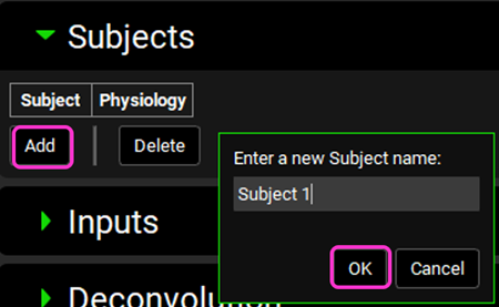
9. Expand the Subjects panel by double-clicking on the panel header bar or clicking on the green arrow.

10. In GPX™ you have the flexibility to deconvolute individual C_p-Time profiles at once. If you wish to do so, you can create an entry for each subject. Since we are dealing with an average C_p-Time profile in this tutorial, we will create just one subject.

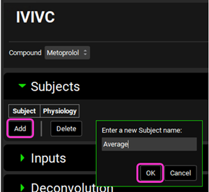
11. Click on Add. The Enter a new Subject name dialog box will appear. Type “Average” and then click OK.

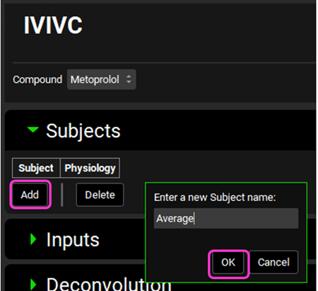
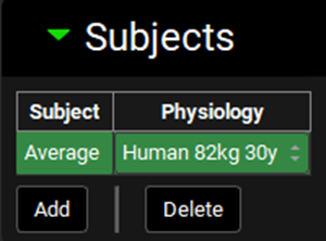
12. A subject entry will be created. In the Physiology drop-down you can select which physiology you wish to link to that subject. Since this project only has one physiology (Human 30YO 66kg), that physiology will be automatically linked to the “Average” subject.

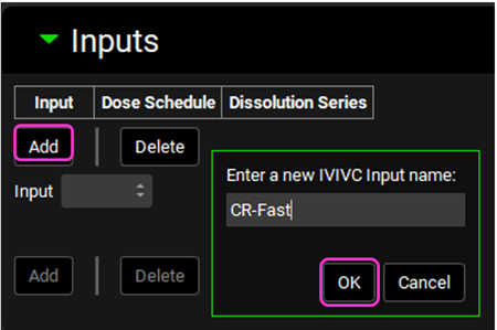
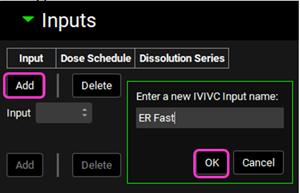
13. Expand the Inputs panel. We will create one input for each formulation in this project, i.e.: CR-Fast; CR-Moderate; CR-Slow and CR-New Form. Click Add to create an input, the Enter a new IVIVC Input name dialog box will appear. Type “CR-Fast” and then click OK.

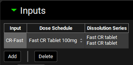
14. After the input is created, the Dose Schedule and Dissolution Series that relates to that input needs to be properly linked. From the Dose Schedule drop-down, select “Fast CR Tablet 100mg” and from the Dissolution Series drop-down select “Fast CR tablet”.

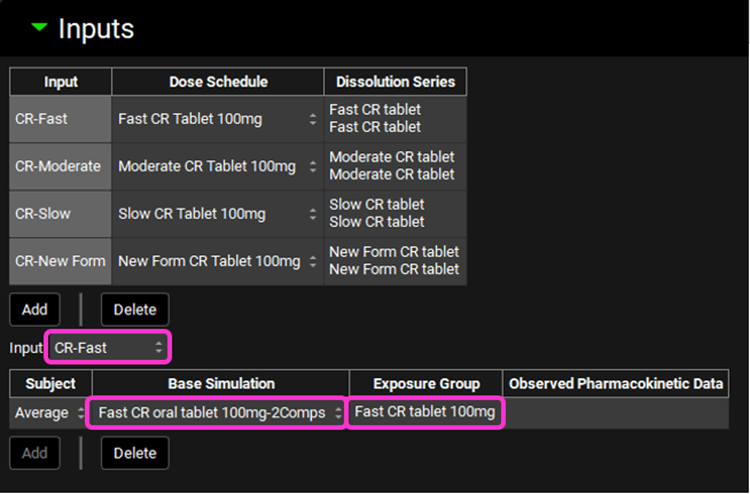
15. Repeat steps 13 and 14 for “CR-Moderate”; “CR-Slow” and “CR-New Form” according to the table below:

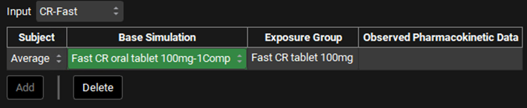
16. Now we will link each input to its associated Base Simulation and C_p-Time data. Select CR-Fast from the Input drop-down. Since we have created only one subject that represents the average profile, that will be the only selection available in the Subject drop-down. In the Base Simulation, select Fast CR oral tablet 100mg-2Comps; and in the Exposure Group drop-down select Fast CR tablet 100mg.

17. Repeat step 16 for CR-Moderate; CR-Slow and CR-New Form according to the table below:

18. Save the project and click OK.

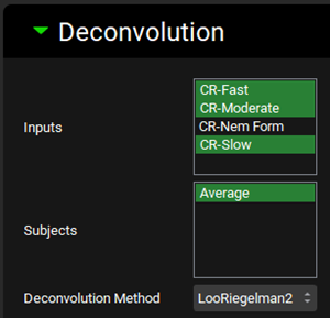
19. Expand the Deconvolution panel. For this example, we will run the Loo-Riegelman (2-compartment model) deconvolution method using the data from both Slow and Moderate formulations. Select CR-Moderate and CR-Slow from the Inputs frame and select Average from the Subjects frame. Select Loo-Riegelman2 from the Deconvolution Method drop-down.

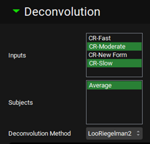
You can also use only one input or as many additional inputs as you like for which you have both in vitro dissolution and oral plasma concentration-time data.

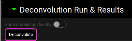
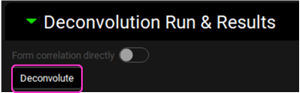
20. Now, you are ready to run the deconvolutions and form a correlation. Expand the Deconvolution Run & Results sub-panel and click on Deconvolute.

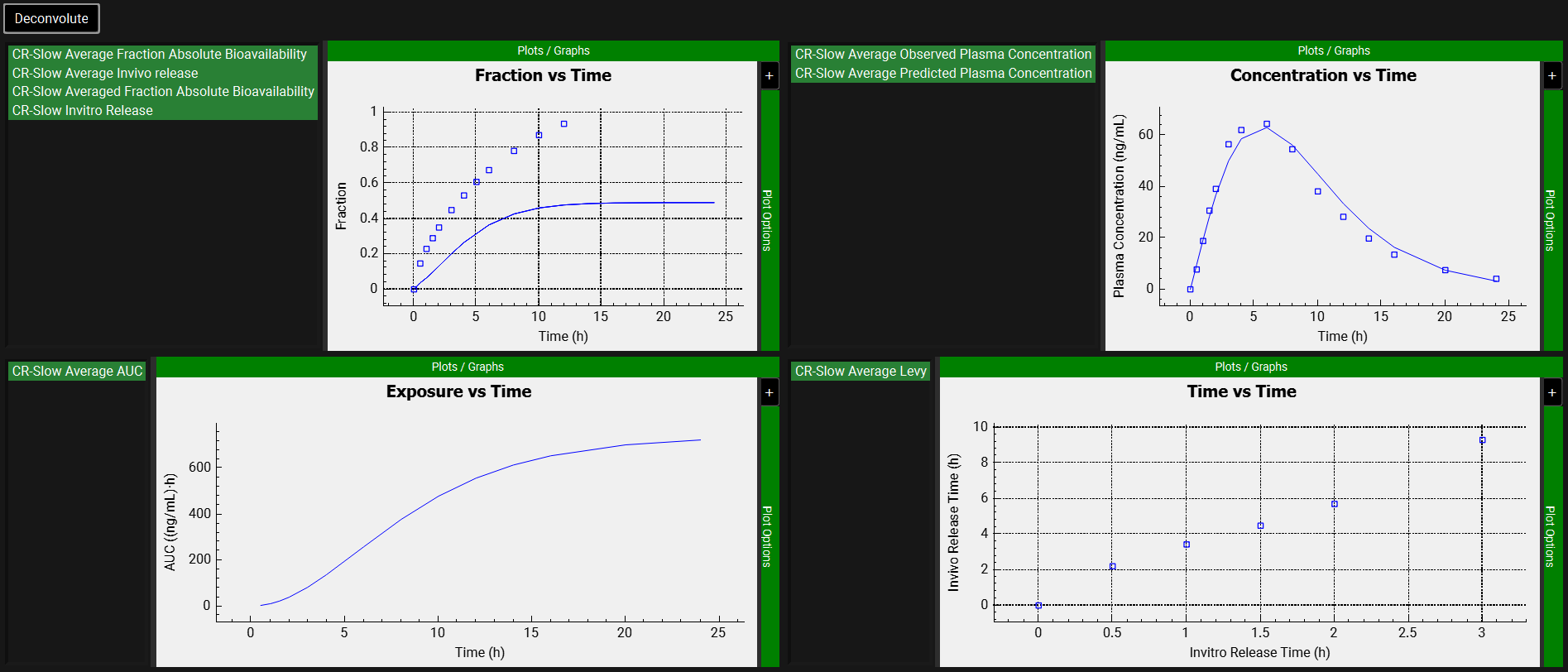
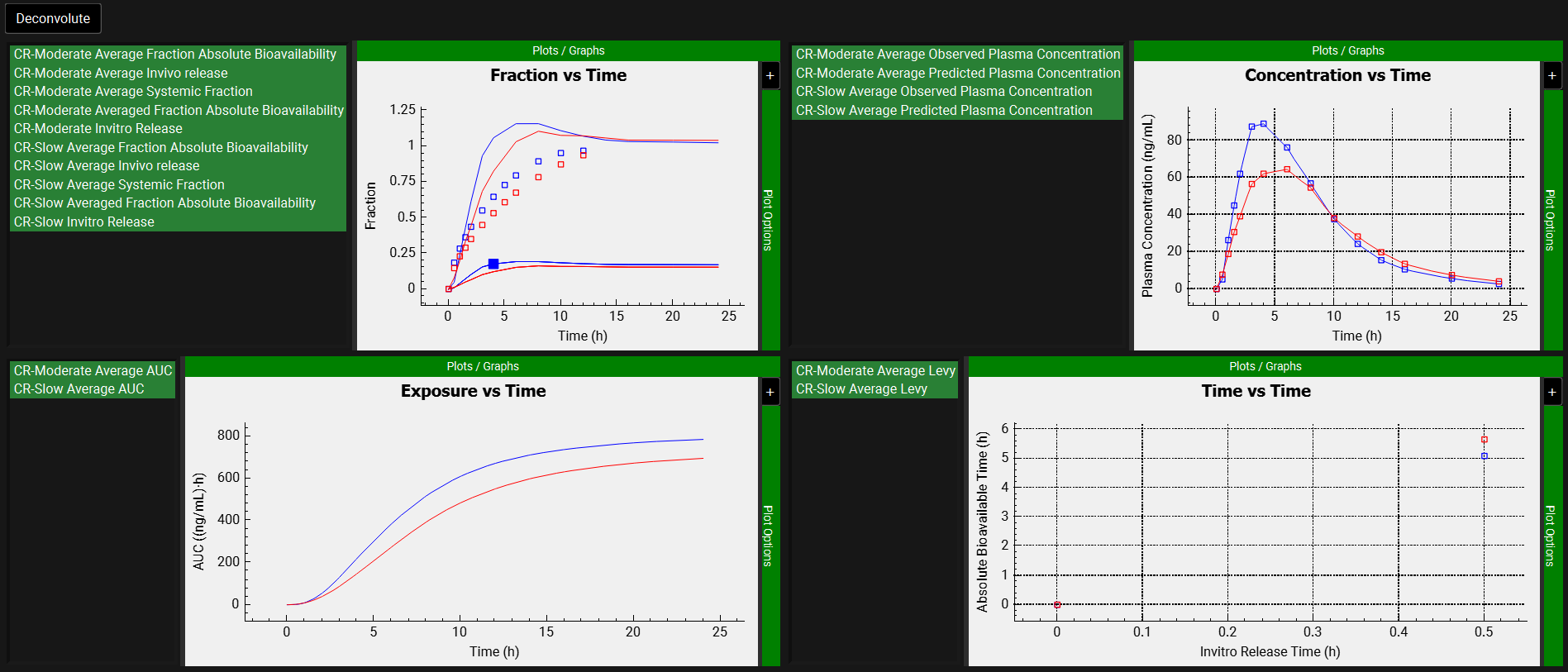
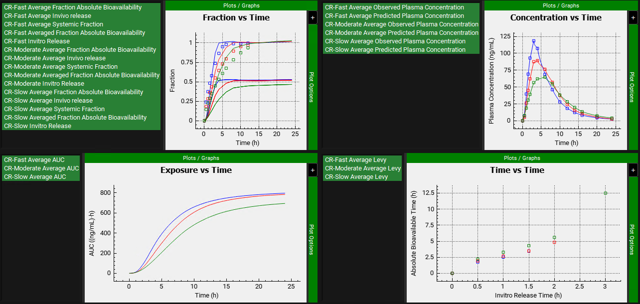
21. After the deconvolution is complete, you will see four graphs. The top-left graph displays 5 types of curves vs time for each input: Fraction Absolute Bioavailability, In vivo release, Systemic Fraction, Averaged Fraction Absolute Bioavailability (in case the multiple subjects deconvolution was performed) and In vitro release. The graph on the top-right displays the deconvoluted profiles for each input. The graph on the bottom-left displays AUC vs. Time for each input and the graph on the bottom-right is a Levy plot.

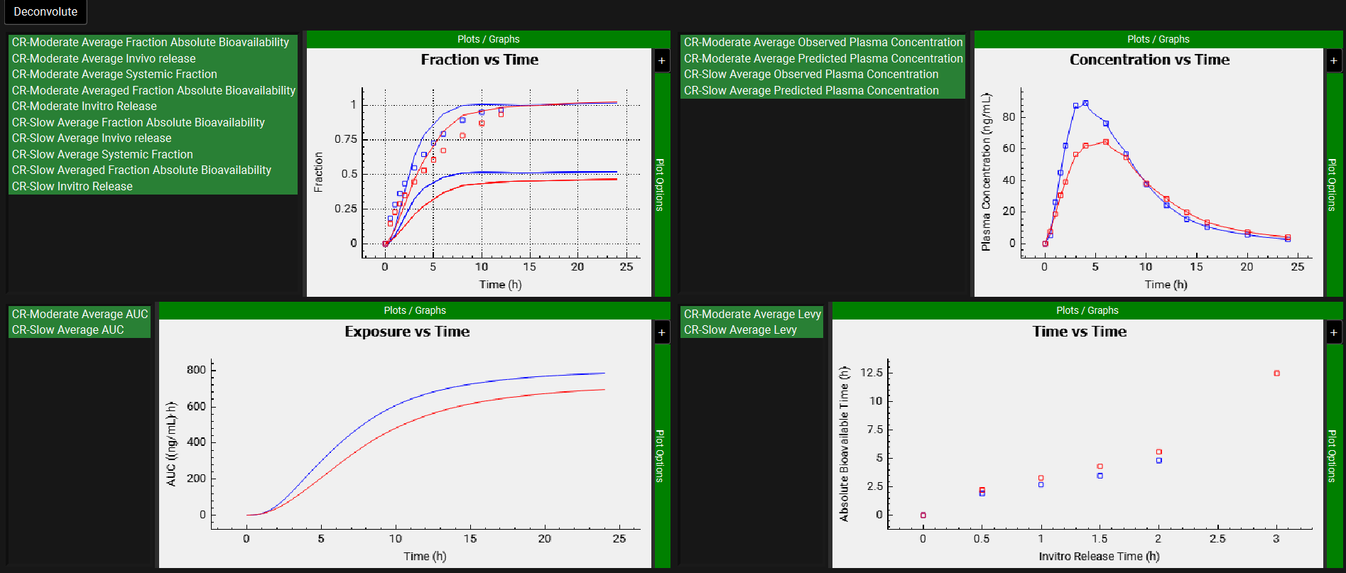
Looking at the deconvolution graph (top-right) we can readily see that there is good agreement between the observed data and the reconstructed plasma Concentration vs Time profiles using the raw deconvoluted Fraction absolute bioavailability vs Time profile.

This is not the predicted plasma concentration-time profile using the absolute bioavailability profile calculated from the in vitro-in vivo correlation, which will be done in the Convolution panel.

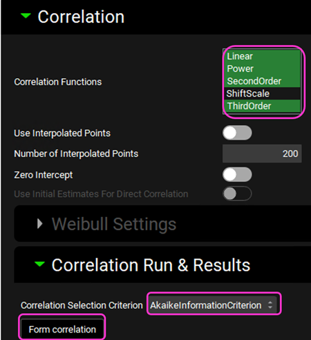
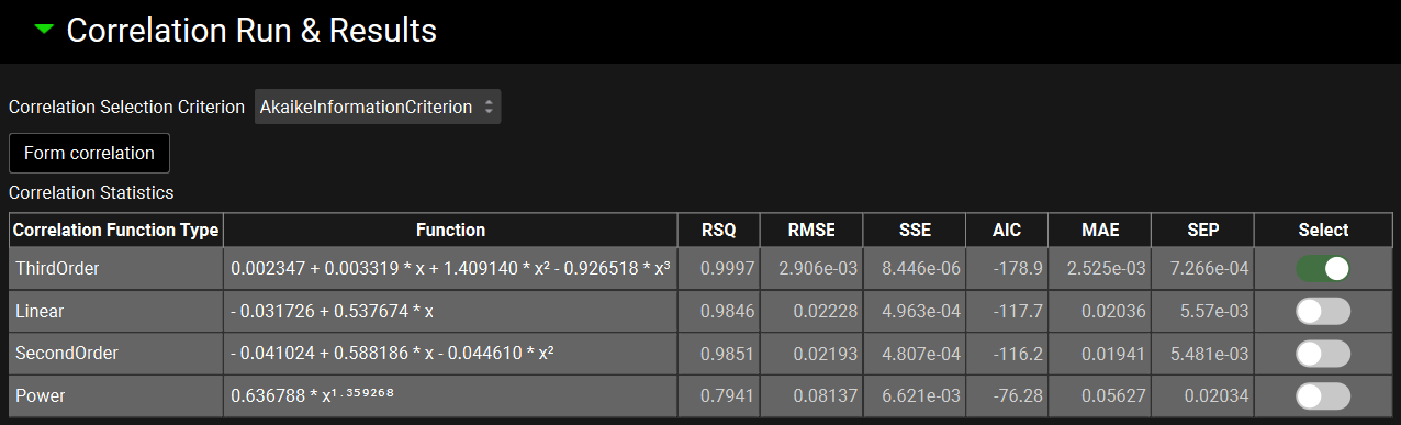
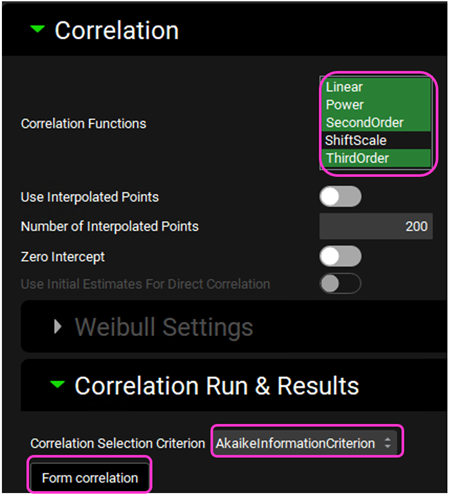
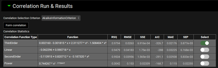
22. Expand the Correlation panel. In the Correlation Functions frame you can select the correlation functions you want to try to fit to the data. For this example, we will select Linear, Power, SecondOrder, and ThirdOrder functions. Scroll down and expand the Correlation Run & Results sub-panel. All checked Correlation Functions will be fitted to the data and the program will pick the best fit based on the Correlation Selection Criterion chosen in this sub-panel. Leave the Akaike Information Criterion selected. Click on the Form Correlation button.

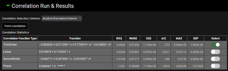
23. The Correlation Statistics table will be displayed when the program is finished fitting all the correlation functions. The best fit (based on the selected criterion) will have the Select toggle on. In this example, a Third Order function was the best.

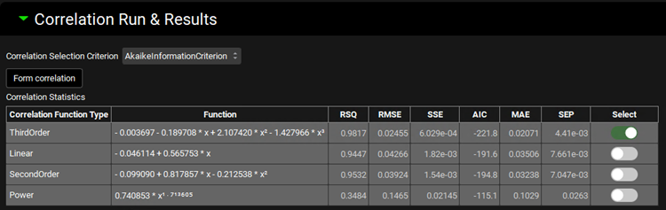
The Correlation Statistics table gives the following information about each correlation: RSQ=R2, RMSE=Root Mean Squared Error; SSE: Sum of Squares Error, AIC=Akaike Information Criterion, MAE=Mean Absolute Error, and SEP=Standard Error of Prediction.

24. The graph below the Correlation Statistics table displays the Fraction Absolute Bioavailability vs Fraction In Vitro Release plot and all fitted correlations. You can hover over each Fitted Series on the left-hand side of the graph for it to be highlighted in the plot.

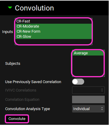
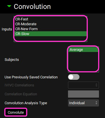
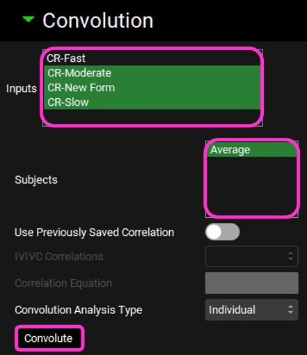
25. Scroll down and expand the Convolution panel. Note that all the inputs are available in the Inputs frame. Select CR-Slow, CR-Moderate, and CR-New Form. In the Subjects frame, select Average and then click on Convolute.

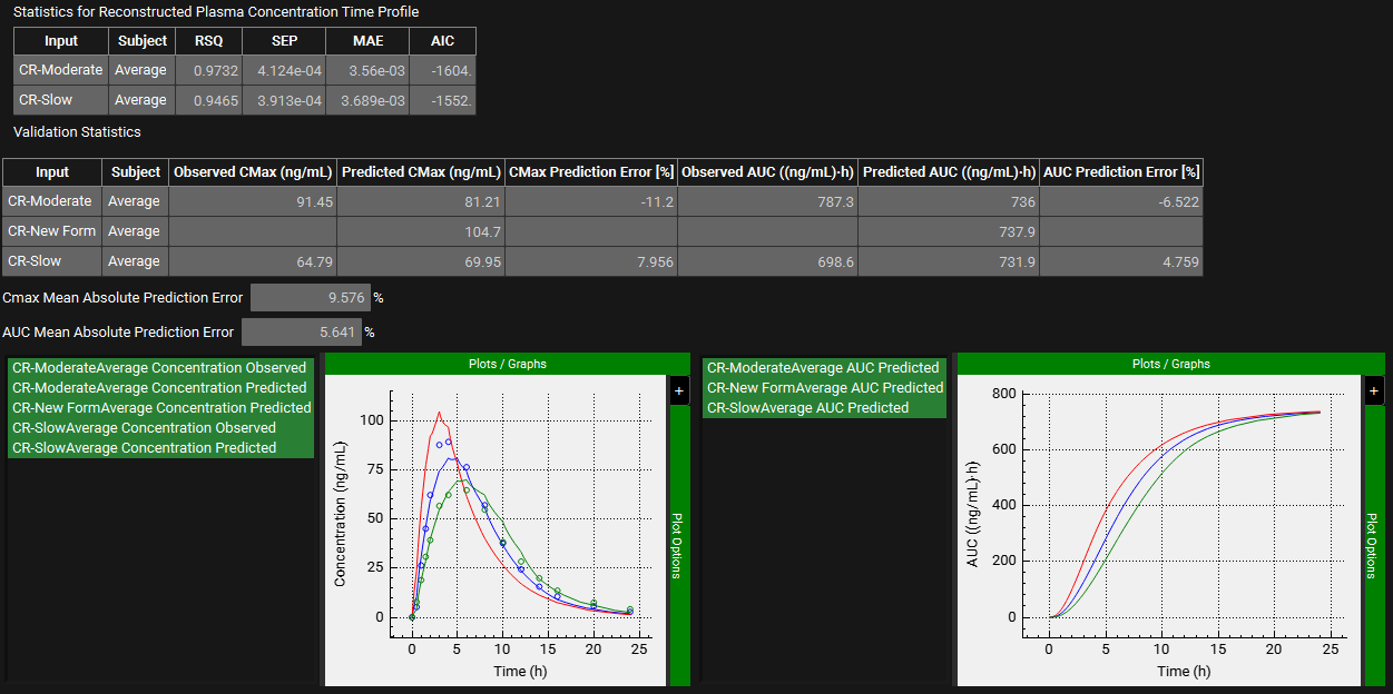
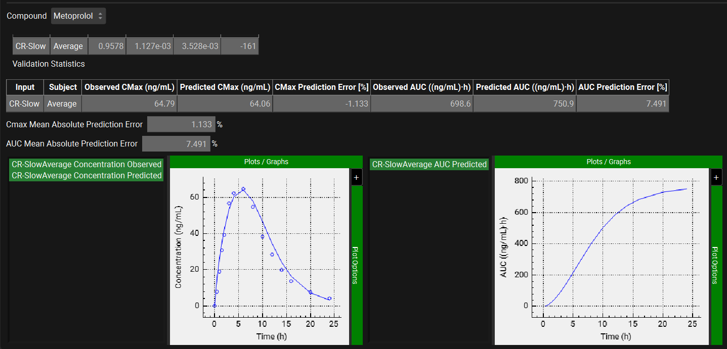
26. When the convolution is finished the observed and predicted plasma concentration-time profiles using the correlation function for all selected inputs will be shown in the left-hand side plot.

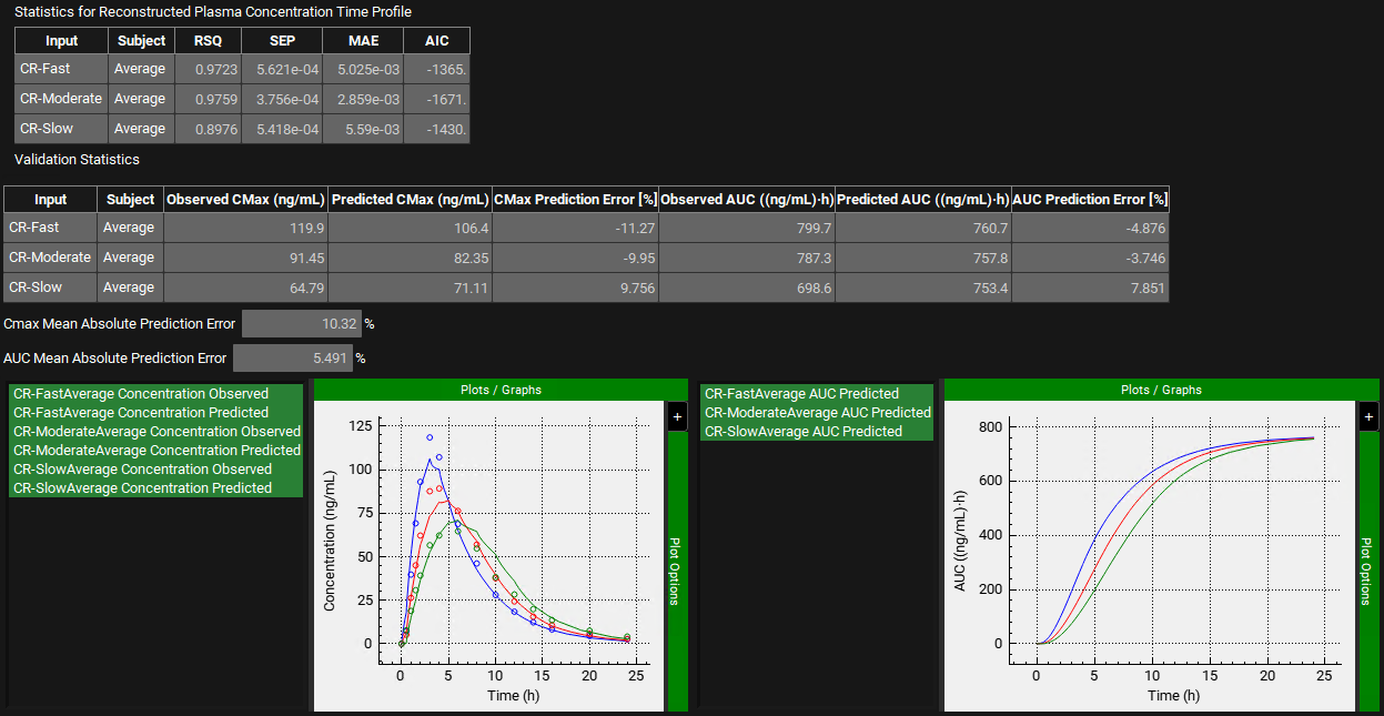
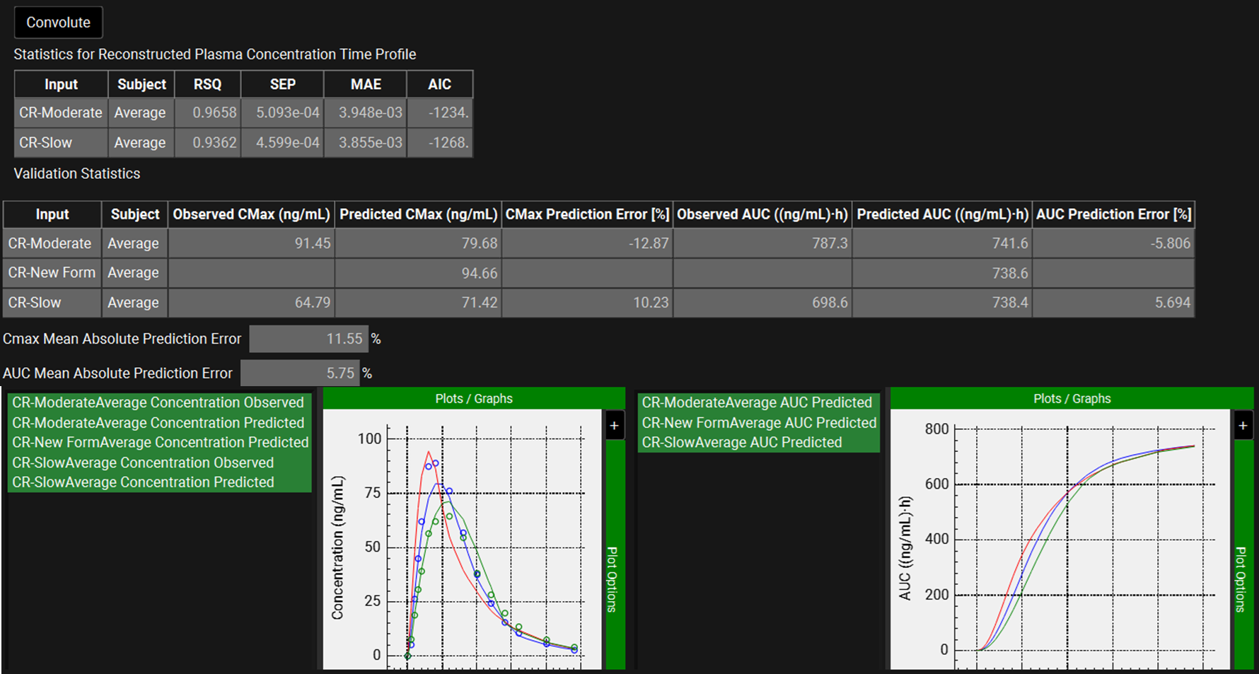
The statistics for the fit of the predicted plasma concentration-time profile using the correlation function to the observed data points will be shown in the Statistics for Reconstructed Plasma Concentration Time Profile table. (RSQ=R2, SEP=Standard Error of Prediction, MAE=Mean Absolute Error, and AIC=Akaike Information Criterion).

The Validation Statistics table will show for each input, the Observed and Predicted values and the percent Prediction Error for C_max and AUC_{(0 to t)}.

The C_max and AUC_{(0 to t)} Mean Absolute Prediction Error % are displayed below the table.

Only drug inputs with a linked exposure data are included in the Mean Absolute Prediction Error % calculation.

These tables may be copied by right clicking on them and then the data pasted into Microsoft Excel.

Numerical Deconvolution

This example illustrates the use of the Numerical Deconvolution method for IVIVC development. 

1. Be sure that you have run Example 1 above before continuing.

2. Open GPX™ and, in the Dashboard view, click on the icon next to Select to open an Existing project.

3. Click Browse and navigate to the C:\Users\<user>\AppData\Local\Simulations Plus, Inc\GastroPlus\10.2\Tutorials\Metoprolol-IVIVC folder and select the project file Metoprolol.gpproject by clicking on it and clicking Open.

4. Navigate to the Pharmacokinetics view and note how there are two pharmacokinetic models linked to the Metoprolol compound: One compartment and Two compartments.

5. Navigate to the Simulations view. Click on the Simulations drop-down to see the simulations in this project. Note how there are two simulations for each formulation: one linked to the One compartment PK model (simulation name with “1Comp” ending) and another with the two Compartments PK model (simulation name with “2Comps” ending).

6. Select any of the “2Comps” simulations and expand the Compound Settings panel. Note that the Compartmental Model Name linked to it is “Two Compartments”. In this tutorial we will be using the “2Comps” simulations as the Base Simulation in IVIVCPlus^™ (explained in more detail in later steps).

7. Click on IVIVCPlus™ in the Modules pane located on the right-hand side of the interface.

8. Expand the Deconvolution panel. For this example, we will run a Numerical deconvolution method using the data from only the Slow formulation. Select CR-Slow from the Inputs frame and select Average from the Subjects frame. Select Numerical from the Deconvolution Method drop-down.

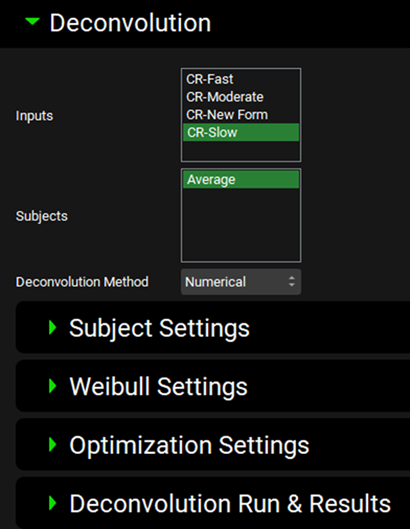
9. When Numerical Deconvolution is selected, the Subject Settings, Weibull Settings, Optimization Settings, and Deconvolution Run & Results sub-panels are enabled.

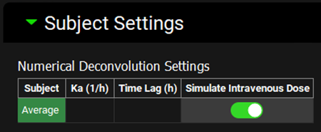
10. Expand the Subject Settings sub-panel to see the Numerical Deconvolution Settings. The Ka (absorption rate constant) and Time Lag (Tlag) parameters, in addition to the ones on the Pharmacokinetics view, are for describing the C_p-Time profile of an oral solution or rapidly dissolving dosage form. If the pharmacokinetic parameters are from an IV administration, the Simulate Intravenous Dose toggle should be on.

11. In this tutorial, the PK parameters were obtained from an IV dose. Select the Simulate Intravenous Dose toggle.

Ka and Tlag can be obtained using the PKPlus™ module. When the simplified absorption parameters are exported to a simulation from PKPlus™, the Ka and Tlag parameter values, if fitted, will be recorded in that simulation. When that simulation is selected as the Base Simulation for an Input in IVIVCPlus™, the values of Ka and Tlag will be automatically loaded. You can also enter these values manually in the Subject Settings sub-panel.

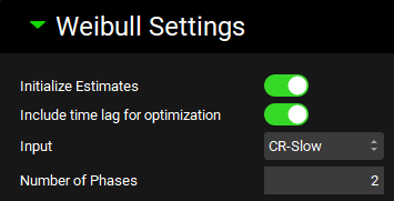
12. Expand the Weibull Settings sub-panel. Click on the Initialize Estimates and Include time lag toggles. Type “2” in the Number of Phases box.

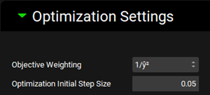
13. Expand the Optimization Settings sub-panel. Here you can choose which Objective Weighting and Optimization Initial Step Size to use for the Weibull fitting. Leave the default selections of 1/ŷ² and 0.05.

14. Now, you are ready to run the deconvolutions and form a correlation. Expand the Deconvolution Run & Results sub-panel and click on Deconvolute.

15. After the deconvolution is complete, you will see four graphs. The top-left graph displays 4 types of curves vs time for each input: Fraction Absolute Bioavailability, In vivo release, Averaged Fraction Absolute Bioavailability (in the case multiple subjects, deconvolution was performed) and In vitro release. The graph on the top-right displays the deconvoluted profiles for each input. The graph on the bottom-left displays AUC vs. Time for each input and the graph on the bottom-right is a Levy plot.

16. Looking at the deconvolution graph (top-right) we can readily see that there is good agreement between the observed data and the reconstructed plasma Concentration vs Time profile using the raw deconvoluted Fraction absolute bioavailability vs Time profile.

This is not the predicted plasma concentration-time profile using the absolute bioavailability profile calculated from the in vitro-in vivo correlation, which will be done in the Convolution panel.

17. Expand the Correlation panel. In the Correlation Functions frame you can select the correlation functions you want to try to fit to the data. For this example, we will select Linear, Power, SecondOrder, and ThirdOrder functions. Scroll down and expand the Correlation Run & Results sub-panel. All checked Correlation Functions will be fitted to the data and the program will pick the best fit based on the Correlation Selection Criterion chosen in this sub-panel. Leave the Akaike Information Criterion selected. Click on the Form Correlation button.

18. The Correlation Statistics table will be displayed when the program is finished fitting all the correlation functions. The best fit (based on the selected criterion) will have the Select toggle on. In this example, a Third Order function was the best.

The Correlation Statistics table gives the following information about each correlation: RSQ=R2, RMSE=Root Mean Squared Error; SSE: Sum of Squares Error, AIC=Akaike Information Criterion, MAE=Mean Absolute Error, and SEP=Standard Error of Prediction.

19. The graph below the Correlation Statistics table displays the Fraction Absolute Bioavailability vs Fraction In Vitro Release plot and all fitted correlations. You can hover over each Fitted Series on the left-hand side of the graph for it to be highlighted in the plot.

20. Scroll down and expand the Convolution panel. Note that all the inputs are available in the Inputs frame. Select CR-Slow. In the Subjects frame, select Average and then click on Convolute.

21. When the convolution is finished the observed and predicted plasma concentration-time profiles using the correlation function for the selected input will be shown in the left-hand side plot.

The statistics for the fit of the predicted plasma concentration-time profile using the correlation function to the observed data points will be shown in the Statistics for Reconstructed Plasma Concentration Time Profile table. (RSQ=R2, SEP=Standard Error of Prediction, MAE=Mean Absolute Error, and AIC=Akaike Information Criterion).

The Validation Statistics table will show for each input, the Observed and Predicted values and the percent Prediction Error for C_max and AUC_{(0 to t)}.

The C_max and AUC_{(0 to t)} Mean Absolute Prediction Error % are displayed below the table.

Only drug inputs with a linked exposure data are included in the Mean Absolute Prediction Error % calculation.

These tables may be copied by right clicking on them and then the data pasted into Microsoft Excel.

Wagner-Nelson (1-compartment model)

This example shows how to use the Wagner-Nelson deconvolution method with the Wagner-Nelson Elimination Rate Constant Estimator. 

1. Be sure that you have run Example 1 above before continuing.

2. Open GPX™ and, in the Dashboard view, click on the icon next to Select to open an Existing project.

3. Click Browse and navigate to the C:\Users\<user>\AppData\Local\Simulations Plus, Inc\GastroPlus\10.2\Tutorials\Metoprolol-IVIVC folder and select the project file Metoprolol.gpproject by clicking on it and clicking Open.

4. Navigate to the Pharmacokinetics view and note how there are two pharmacokinetic models linked to the Metoprolol compound: One compartment and Two compartments.

5. In the One compartment model the clearance is set to zero as in this example we will calculate elimination rate (k_el) from the terminal slope of C_p-Time profile rather than using clearance (CL) and central compartment volume (V_c) as was done in the previous example (k_el = CL/V_c). 

In order to be able to perform the Convolution step and obtain C_p-Time profiles, V_c is always required.

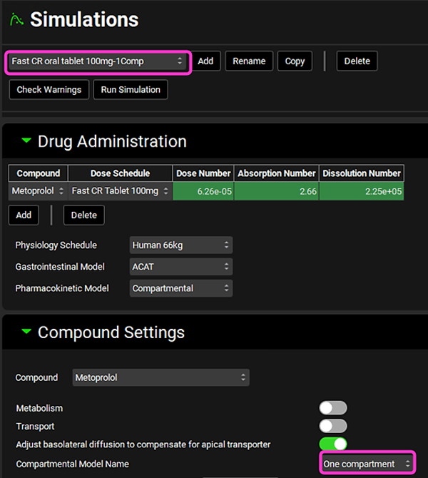
6. Navigate to the Simulations view. Click on the Simulations drop-down to see the simulations in this project. Note how there are two simulations for each formulation: one linked to the One compartment PK model (simulation name with “1Comp” ending) and another with the Two compartments PK model (simulation name with “2Comps” ending).

7. Select any of the “1Comp” simulations and expand the Compound Settings panel. Note that the Compartmental Model Name linked to it is “One compartment”. In this tutorial we will be using the “1Comps” simulations as the Base Simulation in IVIVCPlus™ (explained in more details in later steps) since we are using the Wagner-Nelson deconvolution method.

8. Click on IVIVCPlus™ in the Modules pane located on the right-hand side of the interface. Collapse any opened sub-panels in the Deconvolution panel if they are open.

9. Expand the Inputs panel. Now we will link each input to its associated Base Simulation (1-Comp). The C_p-Time data has already been linked in Example 1. Select CR-Fast from the Input drop-down and in the Base Simulation, select “Fast CR oral tablet 100mg-1Comp”.

10. Repeat step 9 for CR-Moderate; CR-Slow and CR-New Form according to the table below:

11. Save the project and click OK.

12. We will now calculate the elimination rate (k_el) from the terminal slope of the Fast CR tablet C_p-Time profile and export the calculated k_el to each Input. This has to be done for each Input so that the k_el is accounted for when performing Deconvolution and Convolution steps.

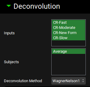
13. Expand the Deconvolution panel and select WagnerNelson1 from the Deconvolution Method drop-down. Then, select all Inputs from the Inputs frame and select Average from the Subjects frame.

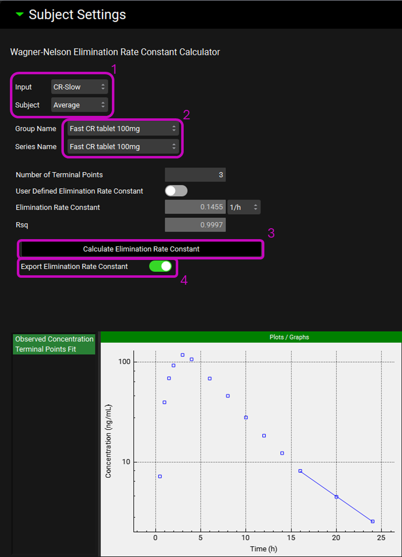
14. Expand the Subjects Settings sub-panel to see the Wagner-Nelson Elimination Rate Constant Calculator. Select CR-Slow from the Input drop-down. The Average subject will be automatically selected. Select Fast CR tablet 100mg from the Group Name drop-down. The k_el will be calculated from this C_p-Time profile. For this example, leave the Number of Terminal Points at three. Click on the Calculate Elimination Rate Constant button. The calculated Elimination Rate Constant and Rsq statistic for the fit will appear in their respective boxes above the Calculate Elimination Rate Constant button and the graph with the fitting will be displayed below. Click on the Export Elimination Rate Constant toggle.

15. Repeat step 14 for all the other Inputs (CR-Fast, CR-Moderate, and CR-New Form).

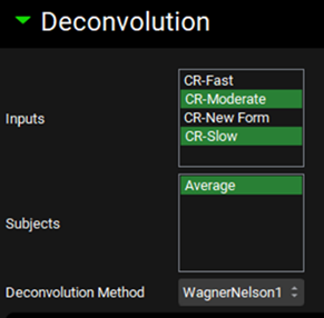
16. For this example, we will run the deconvolution using the data from both Slow and Moderate formulations. Scroll up to the Deconvolution panel and leave only CR-Moderate and CR-Slow selected from the Inputs frame. 

17. Scroll down and expand the Deconvolution Run & Results sub-panel and click on Deconvolute.

18. After the deconvolution is complete, you will see four graphs. The top-left graph displays 5 types of curves vs time for each input: Fraction Absolute Bioavailability, In vivo release, Systemic Fraction, Averaged Fraction Absolute Bioavailability (in the case multiple subjects deconvolution was performed) and In vitro release. The graph on the top-right displays the deconvoluted profiles for each input. The graph on the bottom-left displays AUC vs Time for each input and the graph on the bottom-right is a Levy plot.

Looking at the deconvolution graph (top-right) we can readily see that there is good agreement between the observed data and the reconstructed plasma Concentration-Time profiles using the raw deconvoluted Fraction absolute bioavailability vs Time profile.

This is not the predicted plasma concentration-time profile using the absolute bioavailability profile calculated from the in vitro-in vivo correlation, which will be done in the Convolution panel.

19. Expand the Correlation panel. In the Correlation Functions frame you can select the correlation functions you want to try to fit to the data. For this example, we will select Linear, Power, SecondOrder and ThirdOrder functions. Scroll down and expand the Correlation Run & Results sub-panel. All checked Correlation Functions will be fitted to the data and the program will pick the best fit based on the Correlation Selection Criterion chosen in this sub-panel. Leave the Akaike Information Criterion selected. Click on the Form Correlation button.

20. The Correlation Statistics table will be displayed when the program is finished fitting all the correlation functions. The best fit (based on the selected criterion) will have the Select toggle on. In this example, a Third Order function was the best.

The Correlation Statistics table gives the following information about each correlation: RSQ=R2, RMSE=Root Mean Squared Error; SSE: Sum of Squares Error, AIC=Akaike Information Criterion, MAE=Mean Absolute Error, and SEP=Standard Error of Prediction.

21. The graph below the Correlation Statistics table displays the Fraction Absolute Bioavailability vs Fraction In Vitro Release plot and all fitted correlations. You can hover over each Fitted Series on the left-hand side of the graph for it to be highlighted in the plot.

22. Scroll down and expand the Convolution panel. Note that all the inputs are available in the Inputs frame. Select CR-Slow, CR-Moderate, and CR-New form. In the Subjects frame, select Average and then click on Convolute.

23. When the convolution is finished the observed and predicted plasma concentration-time profiles using the correlation function for all selected inputs will be shown in the left-hand side plot.

The statistics for the fit of the predicted plasma concentration-time profile using the correlation function to the observed data points will be shown in the Statistics for Reconstructed Plasma Concentration Time Profile table. (RSQ=R2, SEP=Standard Error of Prediction, MAE=Mean Absolute Error, and AIC=Akaike Information Criterion).

The Validation Statistics table will show for each input, the Observed and Predicted values and the percent Prediction Error for C_max and AUC_{(0 to t)}.

The C_max and AUC_{(0 to t)} Mean Absolute Prediction Error % are displayed below the table.

Only drug inputs with a linked exposure data are included in the Mean Absolute Prediction Error % calculation.

These tables may be copied by right clicking on them and then the data pasted into Microsoft Excel.

Mechanistic Absorption Model – Two Steps: Deconvolute Then Correlate

The Mechanistic Absorption Model (referred to as Mechanistic in this tutorial) deconvolution method provides a state-of-the-art methodology for performing in vitro – in vivo correlations that is not limited by simplifying assumptions such as linear kinetics and constant absorption rate. By using the full GastroPlus® Advanced Compartmental and Transit (ACAT) model for the oral dosage forms, complex behaviors that include regionally dependent absorption, pH-dependent solubility, precipitation, influx and efflux transport, and saturable systemic and gut metabolism are automatically included in the deconvolution when necessary.

With this method, GastroPlus® can fit the in vivo release-time profile as either a single, double, or triple Weibull function. The optimized Weibull parameters are those that describe in vivo release as a function of time. After the in vivo release is fitted, a correlation function is then fitted between the in vivo release and in vitro release profiles.

In this example, the two steps Mechanistic deconvolution method (Deconvolute and then Correlate) IVIVC Procedure will be used to fit the in vivo release of valproic acid. The parameters of a single Weibull function will be fitted for the deconvolution. A polynomial correlation function will be used to generate an IVIVC.

1. Open GPX™ and, in the Dashboard view, click on the icon next to Select to open an Existing project.

2. Click Browse and navigate to the C:\Users\<user>\AppData\Local\Simulations Plus, Inc\GastroPlus\10.2\Tutorials\Valproate folder and select the project file Valproate.gpproject by clicking on it and clicking Open.

3. Move through the views on the navigation pane from Observed Data to Simulations, observing the information that has been entered in this project.

4. In this project there is one compound (Valproate), one physiology (Human 82kg 30y) and six Extended Release (ER) formulations (ER Fast, ER Medium, ER Medium2, ER Slightly Fast, ER Slightly Slow and ER Slow) with their respective Dosing Schedules. You will also notice that there is an IV infusion Formulations and Dosing Schedule.

In the Observed Data view, you will notice that there are both Exposure Data and In Vitro Dissolution Release for all ER formulations and IV infusion Exposure Data.

5. Navigate to the Pharmacokinetics view and expand the Compartmental panel to see the compartmental PK parameters that were obtained from the IV infusion data using the PKPlus™ module.

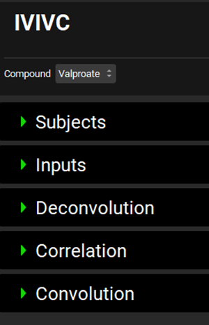
6. Click on IVIVCPlus™ in the Modules pane located on the right-hand side of the interface. The IVIVCPlus™ Module contains five panels: Subjects, Inputs, Deconvolution, Correlation and Convolution.

Expand the Subjects panel by double-clicking on the panel header bar or clicking on the green arrow.

7. In GPX™ you have the flexibility to deconvolute individual C_p-Time profiles at once. If you wish to do so, you can create an entry for each subject. Since we are dealing with an average C_p-Time profile in this tutorial, we will create just one subject.

8. Click on Add. The Enter a new Subject name dialog box will appear. Type “Average” and then click OK (or press Enter).

9. A subject entry will be created. In the Physiology drop-down you can select which physiology you wish to link to that subject. Since this project only has one physiology (Human 82kg 30y), that physiology will be automatically linked to the “Average” subject.

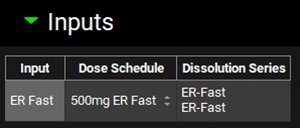
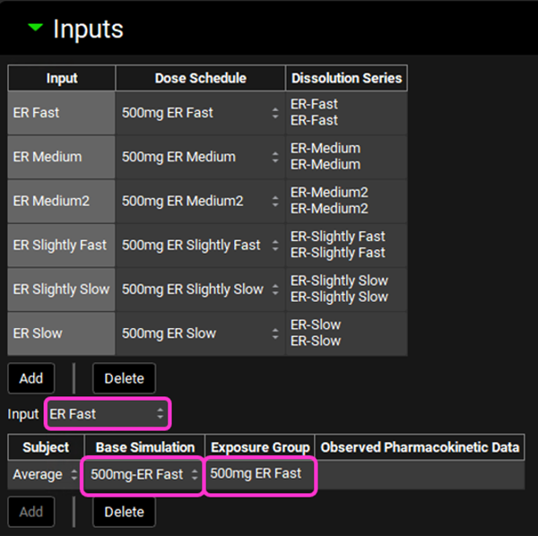
10. Expand the Inputs panel. We will create one input for each formulation in this project, i.e.: ER Fast, ER Medium, ER Medium2, ER Slightly Fast, ER Slightly Slow and ER Slow. Click Add to create an input, the Enter a new IVIVC Input name dialog box will appear. Type “ER Fast” and then click OK.

11. After the input is created, the Dose Schedule and Dissolution Series that relates to that input needs to be properly linked. From the Dose Schedule drop-down, select “500mg ER Fast” and from the Dissolution Series drop-down select “ER-Fast”.

12. Repeat steps 10 and 11 for ER Medium, ER Medium2, ER Slightly Fast, ER Slightly Slow and ER Slow according to the table below:

13. Now we will link each Input to its associated Base Simulation and C_p-Time data, Exposure Group. Select ER Fast from the Input drop-down. Since we have created only one subject that represents the average profile, that will be the only selection available in the Subject drop-down. In the Base Simulation, select 500mg-ER Fast; and in the Exposure Group drop-down select 500mg ER Fast.

14. Repeat step 13 for ER Medium, ER Medium2, ER Slightly Fast, ER Slightly Slow and ER Slow according to the table below:

15. Save the project and click OK.

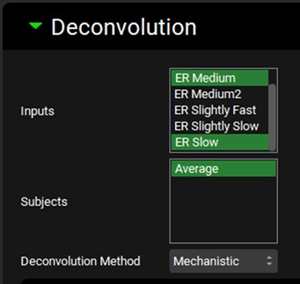
16. Expand the Deconvolution panel. For this example, we will run the Mechanistic deconvolution method using the data from both Medium and Slow formulations. Select ER Medium and ER Slow from the Inputs frame and select Average from the Subjects frame. Select Mechanistic from the Deconvolution Method drop-down.

17. When Mechanistic Deconvolution is selected, the Weibull Settings, Optimization Settings and Deconvolution Run & Results sub-panels are enabled.

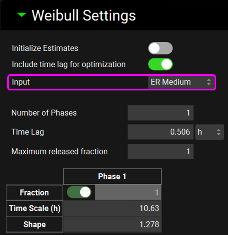
18. Expand the Weibull Settings sub-panel. For this example, we will enter our own initial estimates for fitted parameters in order to speed up the optimization. Uncheck the Initialize Estimates toggle - the Weibull parameters table will be enabled. Leave the Include time lag toggle on. Select ER Medium from the Input drop-down and enter the one phase Weibull parameters for ER Medium according to the table below, you may need to switch the Time Lag units to h:

19. Switch the input to ER Slow and enter the one phase Weibull parameters for the ER Slow according to the table in step 18.

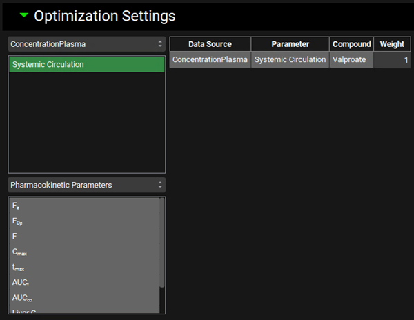
20. Expand the Optimization Settings sub-panel and click on Systemic Circulation in the frame below the ConcentrationPlasma drop-down. An entry will be created in the Optimization Settings table according to this selection. Save the project and click OK.

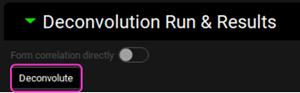
21. Now, you are ready to run the deconvolutions and form a correlation. Expand the Deconvolution Run & Results sub-panel and click on Deconvolute.

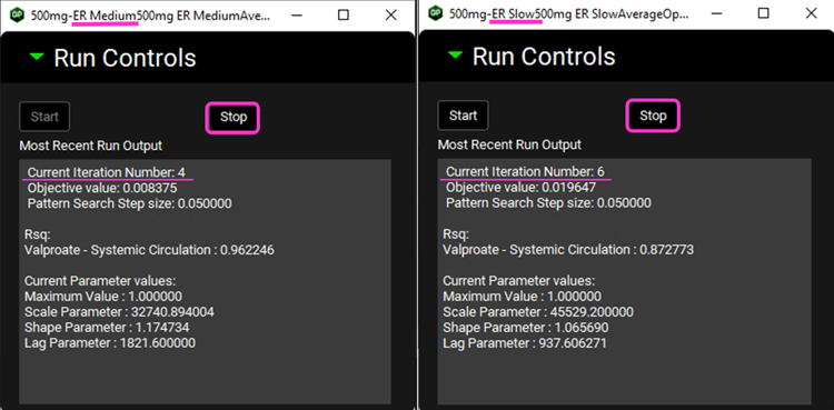
22. The Run Controls window will appear with the optimization status. To save time, we will terminate the optimization early. After a few iterations, click on the Stop button in the Run Controls pop-up after a few iterations. The optimization for the other formulation (the second formulation selected for optimization) will start automatically. Since we have started the optimization with initial values close to the optimum, we can again stop the optimization process early. Click on the Stop button in the Run Controls pop-up after a few iterations.

23. After the deconvolution is complete, you will see four graphs. The top-left graph displays 5 types of curves vs time for each input: Fraction Absolute Bioavailability, In vivo release, Fraction Absorbed, Averaged Fraction Absolute Bioavailability (in case multiple subjects’ deconvolution was performed) and Invitro Release. The graph on the top-right displays the deconvoluted profiles for each input. The graph on the bottom-left displays AUC vs. Time for each input and the graph on the bottom-right is a Levy plot.

In the deconvolution graph (top-right) we can see the reconstructed plasma Concentration-Time profiles (lines) using the deconvoluted Fraction In Vivo Release vs. Time profile.

This is not the in vivo release profile calculated from the in vitro-in vivo correlation, which will be done in the Convolution panel.

Depending on when the deconvolution step was halted, your results may look slightly different to those above.

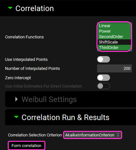
24. Expand the Correlation panel. In the Correlation Functions frame you can select the correlation functions you want to try to fit to the data. For this example, we will select Linear, Power, SecondOrder and ThirdOrder functions. Scroll down and expand the Correlation Run & Results sub-panel. All checked Correlation Functions will be fitted to the data and the program will pick the best fit based on the Correlation Selection Criterion chosen in this sub-panel. Leave the AkaikeInformationCriterion selected. Click on the Form Correlation button.

25. The Correlation Statistics table will be displayed when the program is finished fitting all the correlation functions. The best fit (based on the selected criterion) will have the Select toggle on. In this example, a Third Order function was the best.

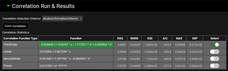
The Correlation Statistics table gives the following information about each correlation: RSQ=R2, RMSE=Root Mean Squared Error; SSE: Sum of Squares Error, AIC=Akaike Information Criterion, MAE=Mean Absolute Error, and SEP=Standard Error of Prediction.

Depending on when the deconvolution step was halted, your results may look slightly different to those above.

26. The graph below the Correlation Statistics table displays the Fraction In Vivo Release vs. Fraction In Vitro Release plot and all fitted correlations. You can hover over each Fitted Series on the left-hand side of the graph for it to be highlighted in the plot.

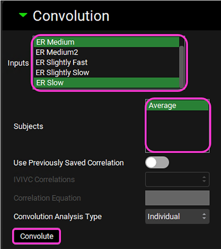
27. Scroll down and expand the Convolution panel. Note that all the inputs are available in the Inputs frame. Select ER Medium and ER Slow. In the Subjects frame, select Average and then click on Convolute.

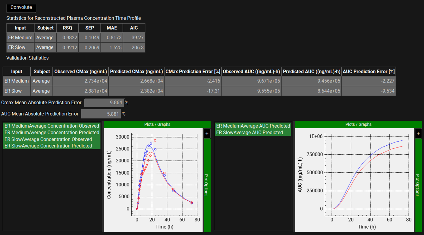
28. When the convolution is finished the observed and predicted plasma Concentration-Time profiles using the correlation function for the selected inputs will be shown in the left-hand side plot.

The statistics for the fit of the predicted plasma Concentration-Time profiles using the correlation function to the observed data points will be shown in the Statistics for Reconstructed Plasma Concentration Time Profile table. (RSQ=R2, SEP=Standard Error of Prediction, MAE=Mean Absolute Error, and AIC=Akaike Information Criterion).

The Validation Statistics table will show for each input, the Observed and Predicted values and the percent Prediction Error for C_max and AUC_{(0 to t)}.

The C_max and AUC_{(0 to t)} Mean Absolute Prediction Error % are displayed below the table.

Only drug inputs with a linked exposure data are included in the Mean Absolute Prediction Error % calculation.

These tables may be copied by right clicking on them and then the data can be pasted into Microsoft Excel.

If you wish to repeat this exercise with different combinations of formulations, you can speed up the optimizations by using the pre-optimized parameters listed in the table below as initial estimates of one phase Weibull parameters for individual formulations.

Multiple Subjects

1. Open GPX™ and, in the Dashboard view, click on the icon next to Select to open an Existing project.

2. Click Browse and navigate to the C:\Users\<user>\AppData\Local\Simulations Plus, Inc\GastroPlus\10.2\Tutorials\Multiple Subjects and select the project file Multiple Subjects.gpproject by clicking on it and clicking Open.

3. Navigate to the Observed Data view and note how there are Exposure Data for 5 subjects and one In Vitro Dissolution Release profile for a Valproate ER formulation.

4. There are 5 different physiologies named after each subject (one through five) in this project which can be viewed in the Physiologies view via the Physiology drop-down.

5. Navigate to the Pharmacokinetics view and note how there are five individual subject pharmacokinetic models linked to the Valproate compound.

6. Navigate to the Simulations view. Click on the Simulations drop-down to see the simulations in this project. Note how there is one simulation for each subject.

7. Select Subject 3 Simulation and expand the Drug Administration and Compound Settings panels, as well as the Observed Data sub-panel. Note that the Physiology Schedule, the Compartmental Model Name, and the Observed Data linked to it is all related to Subject 3. In this tutorial we will be using each subject simulation as a Base Simulation in IVIVCPlus™(explained in more details in later steps).

8. Click on IVIVCPlus™ in the Modules pane located on the right-hand side of the interface and ensure all of the panels are closed.

9. Expand the Subjects panel by double-clicking on the panel header bar or clicking on the green arrow.

10. In GPX™ you have the flexibility to deconvolute individual C_p-Time profiles simultaneously. We will create an entry for each subject.

11. Click on Add. The Enter a new Subject name dialog box will appear. Type “Subject 1” and then click OK (or press Enter).

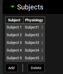
12. A subject entry will be created. In the Physiology drop-down you can select which physiology you wish to link to that subject. From the Physiology drop-down, select Subject1.

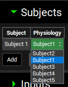
13. Repeat steps 11 and 12 for Subjects 2, 3, 4 and 5 linking each subject input to its corresponding Physiology.

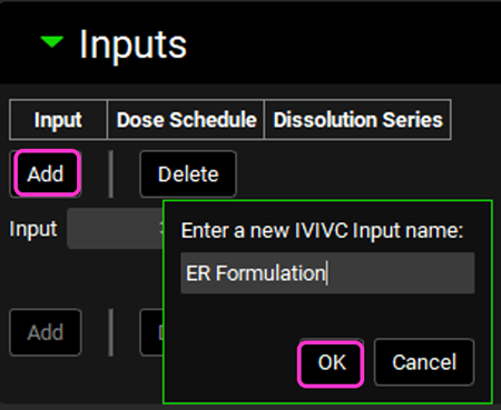
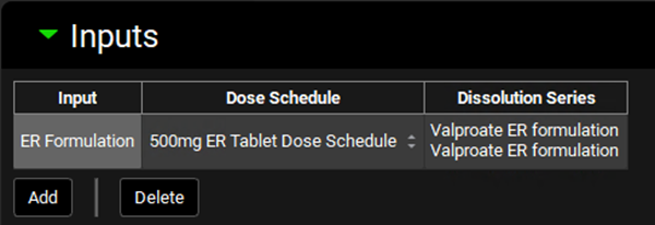
14. Expand the Inputs panel. We will create one input for the formulation in this project, Valproate ER Formulation. Click Add to create an input, the Enter a new IVIVC Input name dialog box will appear. Type “ER Formulation” and then click OK.

15. After the input is created, the Dose Schedule and Dissolution Series that relates to that input needs to be properly linked. Since this project only has one Dose Schedule (500mg ER Tablet Dose Schedule), that schedule will be automatically selected. The same is true for the Dissolution Series.

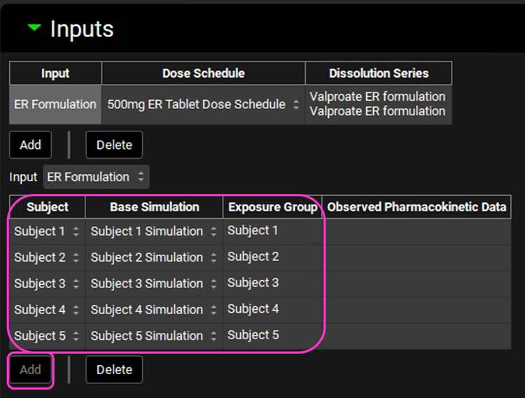
16. Now we will create five subject entries for the ER Formulation input and link each subject to its associated Base Simulation.

Under the Input drop-down table, click Add four times to add all subjects. Once you have created an entry for each subject, the Add button will no longer be available.

Select the Base Simulation and Exposure Group pertaining to each subject as shown in the screenshot below.

17. Save the project and click OK.

18. Expand the Deconvolution panel. For this example, we will run the Loo-Riegelman (2-compartment model) deconvolution method using the data from all subjects. Select ER Formulation from the Inputs frame and select Subjects 1-5 from the Subject frame. Select Loo-Riegelman2 from the Deconvolution Method drop-down.

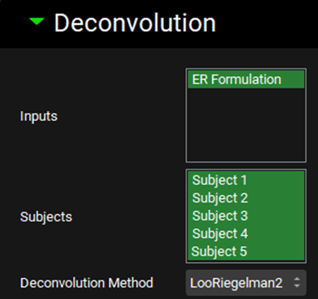
You can also use only one input or as many additional inputs as you like for which you have both in vitro dissolution and oral plasma concentration-time data.

19. Now, you are ready to run the deconvolutions and form a correlation. Expand the Deconvolution Run & Results sub-panel and click on Deconvolute.

20. After the deconvolution is complete, you will see four graphs. The top-left graph displays 3 curves vs time for each Subject: Fraction Absolute Bioavailability, Invivo release and Systemic Fraction. There is also an Averaged Fraction Absolute Bioavailability vs Time curve that represents the average between all selected subjects. And lastly, the Invitro release for the ER Formulation is also displayed. The graph on the top-right displays the deconvoluted profiles for each subject. The graph on the bottom-left displays AUC vs. Time for each subject and the graph on the bottom-right is a Levy plot.

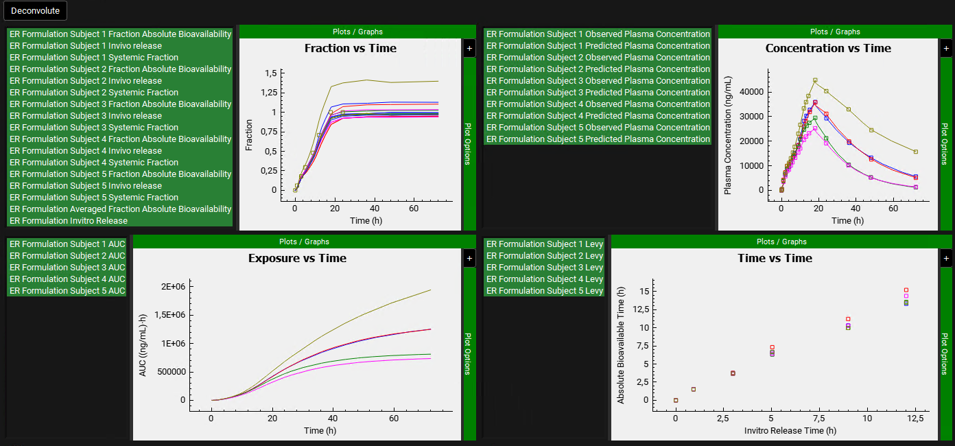
Looking at the deconvolution graph (top-right) we can readily see that there is good agreement between the observed data and the reconstructed plasma Concentration vs Time profiles using the raw deconvoluted Fraction Absolute Bioavailability vs Time profile.

This is not the predicted plasma concentration-time profile using the absolute bioavailability profile calculated from the in vitro-in vivo correlation, which will be done in the Convolution panel.

21. Expand the Correlation panel. In the Correlation Functions frame you can select the correlation functions you want to try to fit to the data. For this example, we will select Linear, Power, SecondOrder and ThirdOrder functions. Scroll down and expand the Correlation Run & Results sub-panel. All checked Correlation Functions will be fitted to the data and the program will pick the best fit based on the Correlation Selection Criterion chosen in this sub-panel. Leave the Akaike Information Criterion selected. Click on the Form Correlation button.

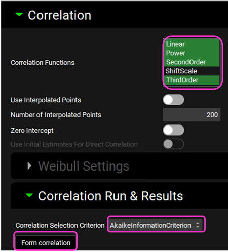
The correlation function is fitted based on the averaged Fraction Absolute Bioavailability vs Fraction In Vitro Release across all subjects. There is a single correlation fitted that represents all subject.

22. The Correlation Statistics table will be displayed when the program is finished fitting all the correlation functions. The best fit (based on the selected criterion) will have the Select toggle on. In this example, a Third Order function was the best.

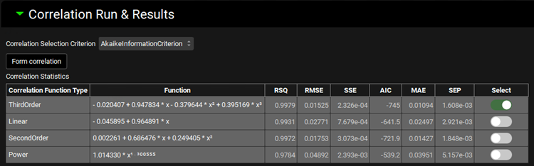
The Correlation Statistics table gives the following information about each correlation: RSQ=R2, RMSE=Root Mean Squared Error; SSE: Sum of Squares Error, AIC=Akaike Information Criterion, MAE=Mean Absolute Error, and SEP=Standard Error of Prediction.

23. The graph below the Correlation Statistics table displays the Fraction Absolute Bioavailability vs Fraction In Vitro Release plot and all fitted correlations. You can hover over each Fitted Series on the left-hand side of the graph for it to be highlighted in the plot.

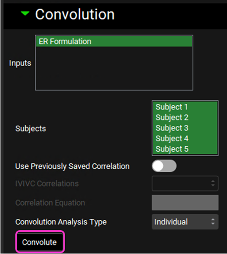
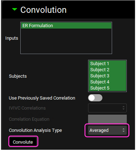
24. Scroll down and expand the Convolution panel. In the Inputs frame, select ER Formulation. Note that all the subjects are available in the Subject frame. Select all subjects. Leave Individual selected in the Convolution Analysis Type drop-down and then click on Convolute.

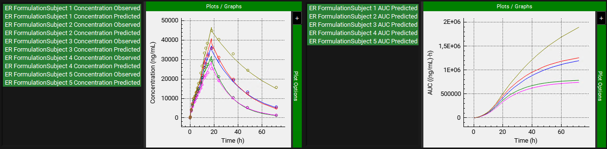
25. When the convolution is finished the observed and predicted plasma concentration-time profiles using the correlation function for each selected subject will be shown in the left-hand side plot.

26. The statistics for the fit of the predicted plasma Concentration-Time profile using the correlation function to the observed data points will be shown in the Statistics for Reconstructed Plasma Concentration Time Profile table. (RSQ=R2, SEP=Standard Error of Prediction, MAE=Mean Absolute Error, and AIC=Akaike Information Criterion).

The Validation Statistics table will show for each input, the Observed and Predicted values and the percent Prediction Error for C_max and AUC_{(0 to t)}.

The C_max and AUC_{(0 to t)} Mean Absolute Prediction Error % are displayed below the table.

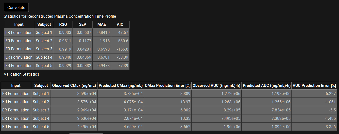
Only drug inputs with a linked exposure data are included in the Mean Absolute Prediction Error % calculation.

These tables may be copied by right clicking on them and then the data can be pasted into Microsoft Excel.

27. Scroll up and select Averaged from the Convolution Analysis Type drop-down and then click on Convolute.

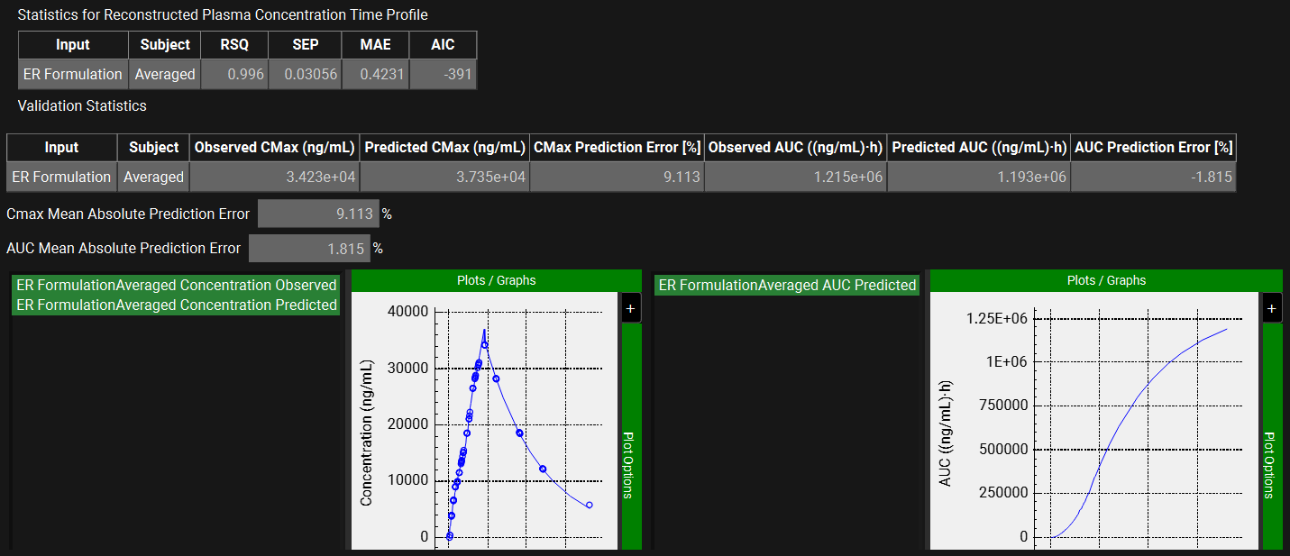
When Averaged is selected the fit statistics will be calculated based on the Averaged Observed vs. Predicted C_p-Time curves (averaged across all subjects selected).

28. When the convolution is finished the observed and predicted plasma Concentration-Time profile using the correlation function for the Averaged profile will be shown in the left-hand side plot.

The statistics for the fit of the predicted plasma Concentration-Time profile using the correlation function to the observed data points will be shown in the Statistics for Reconstructed Plasma Concentration Time Profile table. (RSQ=R2, SEP=Standard Error of Prediction, MAE=Mean Absolute Error, and AIC=Akaike Information Criterion).

The Validation Statistics table will show for the Averaged subject, the Observed and Predicted values and the percent Prediction Error for C_max and AUC_{(0 to t)}.

The C_max and AUC_{(0 to t)} Mean Absolute Prediction Error % are displayed below the table.

These tables may be copied by right clicking on them and then the data can be pasted into Microsoft Excel.

Saving an IVIVC Correlation and Using it to Generate an In Vivo Dissolution Profile

If you have not followed the IVIVCPlus™ module tutorials in order, please refer to the Loo-Riegelman (2-compartment model) section to set up subjects and inputs for this tutorial.

1. Open GPX™ and, in the Dashboard view, click on the icon next to Select to open an Existing project.

2. Click Browse and navigate to the C:\Users\<user>\AppData\Local\Simulations Plus, Inc\GastroPlus\10.2\Tutorials\Save Correlation folder and select the project file Metoprolol IVIVC.gpproject by clicking on it and clicking Open.

3. Move through the views on the navigation pane from Observed Data to Simulations, observing the information that has been entered in this project.

4. In this project there is one compound (Metoprolol), one physiology (Human 30YO 66kg) and four different formulations (Fast CR Tablet, Moderate CR Tablet, Slow CR Tablet and New Form CR Tablet) with their respective Dosing Schedules.

In the Observed Data view, you will notice that there are both Exposure Data and In Vitro Dissolution Release for the Fast, Moderate and Slow formulations, while the New Form formulation only has In Vitro Dissolution Release data.

In the IVIVCPlus™ module, only assets that have both Exposure Data and In Vitro Dissolution Release data can be used for forming correlations. Assets with only In Vitro Dissolution Release data can be used for convolution to predict the likely C_p-Time profiles before dosing in subjects.

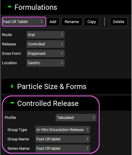
5. Navigate to the Dosing view and expand the Formulations panel by double-clicking on the panel header bar or clicking on the green arrow.

6. Select “Fast CR Tablet” from the drop-down if not already selected and expand the Controlled Release sub-panel.

Since the Release is selected as “Controlled”, the Controlled Release sub-panel is available.

7. From the Profile drop-down you can define the release as Tabulated data or Distribution profile (via Weibull function). Leave Tabulated selected.

8. Click on the Group Type drop-down and note that you can either select In Vitro Dissolution Release or In Vivo Controlled Release. Only In Vitro Dissolution Release data have been entered in the Observed Data, so select In Vitro Dissolution Release. The in vitro dissolution data related to the Fast CR tablet has been already linked in the Group Name and Series Name.

Note how the other formulations have been already linked to their respective in vitro dissolution data by switching the formulation from the Formulations drop-down.

9. Navigate to the Pharmacokinetics view and note how there is a two-compartment pharmacokinetic model linked to the Metoprolol compound.

10. Click on IVIVCPlus™ in the Modules pane located on the right-hand side of the interface.

11. Expand the Subjects and Inputs panels by double-clicking on the panel header bar or clicking on the green arrow. The inputs in these panels have already been created.

12. Expand the Deconvolution panel. For this example, we will run the Loo-Riegelman (2-compartment model) deconvolution method using the data from Slow, Moderate and Fast formulations. The CR-Fast, CR-Moderate and CR-Slow inputs are selected from the Inputs frame and Average from the Subjects frame. The Loo-Riegelman2 method is also selected from the Deconvolution Method drop-down.

13. Expand the Deconvolution Run & Results sub-panel and click on Deconvolute.

14. After the deconvolution is complete, you will see four graphs. The top-left graph displays 5 types of curves vs time for each input: Fraction Absolute Bioavailability, In vivo release, Systemic Fraction, Averaged Fraction Absolute Bioavailability (in case the multiple subjects deconvolution was performed) and In vitro release. The graph on the top-right displays the deconvoluted profiles for each input. The graph on the bottom-left displays AUC vs. Time for each input and the graph on the bottom-right is a Levy plot.

Looking at the deconvolution graph (top-right) we can readily see that there is good agreement between the observed data and the reconstructed plasma Concentration vs Time profiles using the raw deconvoluted Fraction absolute bioavailability vs Time profile.

This is not the predicted plasma concentration-time profile using the absolute bioavailability profile calculated from the in vitro-in vivo correlation, which will be done in the Convolution panel.

15. Expand the Correlation panel. In the Correlation Functions frame you can select the correlation functions you want to try to fit to the data. For this example, we will select Linear, Power, SecondOrder and ThirdOrder functions. Scroll down and expand the Correlation Run & Results sub-panel. All checked Correlation Functions will be fitted to the data and the program will pick the best fit based on the Correlation Selection Criterion chosen in this sub-panel. Leave the Akaike Information Criterion selected. Click on the Form Correlation button.

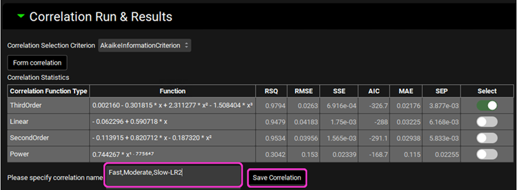
16. The Correlation Statistics table will be displayed when the program is finished fitting all the correlation functions. The best fit (based on the selected criterion) will have the Select toggle on. In this example, a Third Order function was the best.

The Correlation Statistics table gives the following information about each correlation: RSQ=R2, RMSE=Root Mean Squared Error; SSE: Sum of Squares Error, AIC=Akaike Information Criterion, MAE=Mean Absolute Error, and SEP=Standard Error of Prediction.

17. The graph below the Correlation Statistics table displays the Fraction Absolute Bioavailability vs Fraction In Vitro Release plot and all fitted correlations. You can hover over each Fitted Series on the left-hand side of the graph for it to be highlighted in the plot.

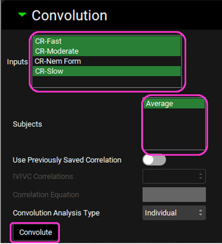
18. Scroll down and expand the Convolution panel. Note that all the inputs are available in the Inputs frame. Select CR-Fast, CR-Moderate and CR-Slow. In the Subjects frame, select Average and then click on Convolute.

19. When the convolution is finished the observed and predicted plasma concentration-time profiles using the correlation function for all selected inputs will be shown in the left-hand side plot.

The statistics for the fit of the predicted plasma concentration-time profile using the correlation function to the observed data points will be shown in the Statistics for Reconstructed Plasma Concentration Time Profile table. (RSQ=R2, SEP=Standard Error of Prediction, MAE=Mean Absolute Error, and AIC=Akaike Information Criterion).

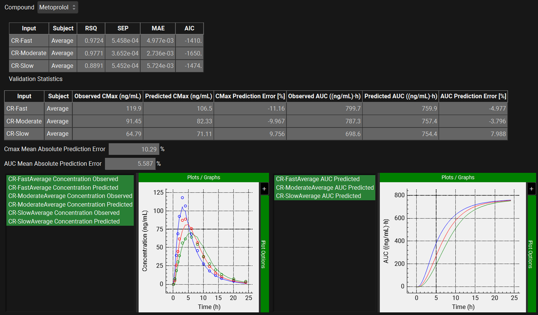
The Validation Statistics table will show for each input, the Observed and Predicted values and the percent Prediction Error for C_max and AUC_{(0 to t)}.

We can see that for each formulation, the C_max and AUC Prediction Errors have not exceeded 15%.

The C_max and AUC_{(0 to t)} Mean Absolute Prediction Error % are displayed below the table. We will consider these values acceptable since the C_max Mean Absolute Prediction Error is ~10% and the AUC Mean Absolute Prediction Error is 5.5% (<10%).

20. We will save this correlation and use it to generate an in vivo dissolution series for the New Form formulation and use it to predict its C_p-Time profile.

21. Scroll up to the Correlation Run & Results panel.

22. Type “Fast,Moderate,Slow-LR2” in the Please specify correlation name box located under the Correlation Statistics table. Click on the Save Correlation button.

23. A message will appear in the Messages center saying that the correlation has been saved and it can be accessed via the Dosing view and IVIVC/Convolution view. Click Done to clear the message.

24. Navigate to the Dosing view. Expand the Formulations panel and select New Form CR Tablet from the drop-down.

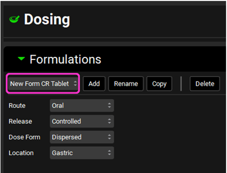
25. Expand the Controlled Release sub-panel, ensure that Group Type is In Vitro Dissolution Release, and select the Use IVIVC Correlation toggle. The Fast,Moderate,Slow-LR2 correlation will be shown in the IVIVC Correlation drop-down and the Correlation Equation is displayed below.

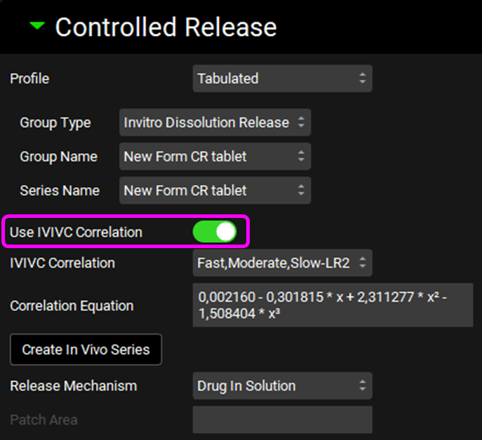
If you have saved more than one correlation (e.g.: with different inputs or different method), they will be shown in the IVIVC Correlation drop-down and you can select from it.

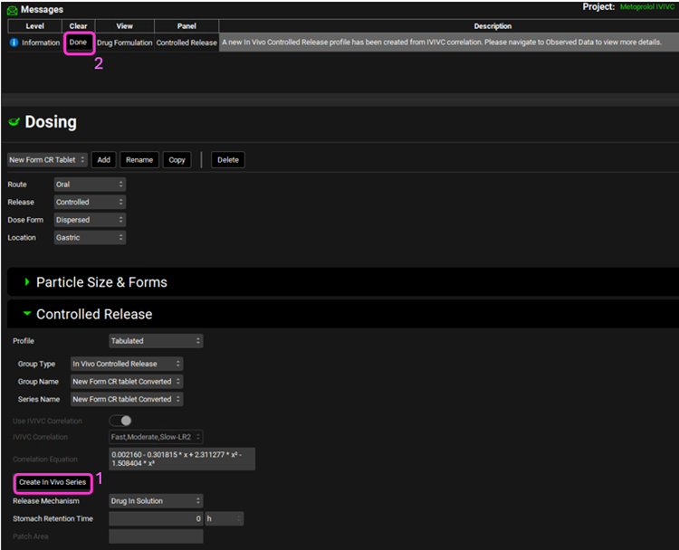
26. Click on Create In Vivo Series. A message will appear in the Messages center informing you that a new In Vivo Controlled Release profile has been created from the IVIVC correlation. Click Done to clear the message.

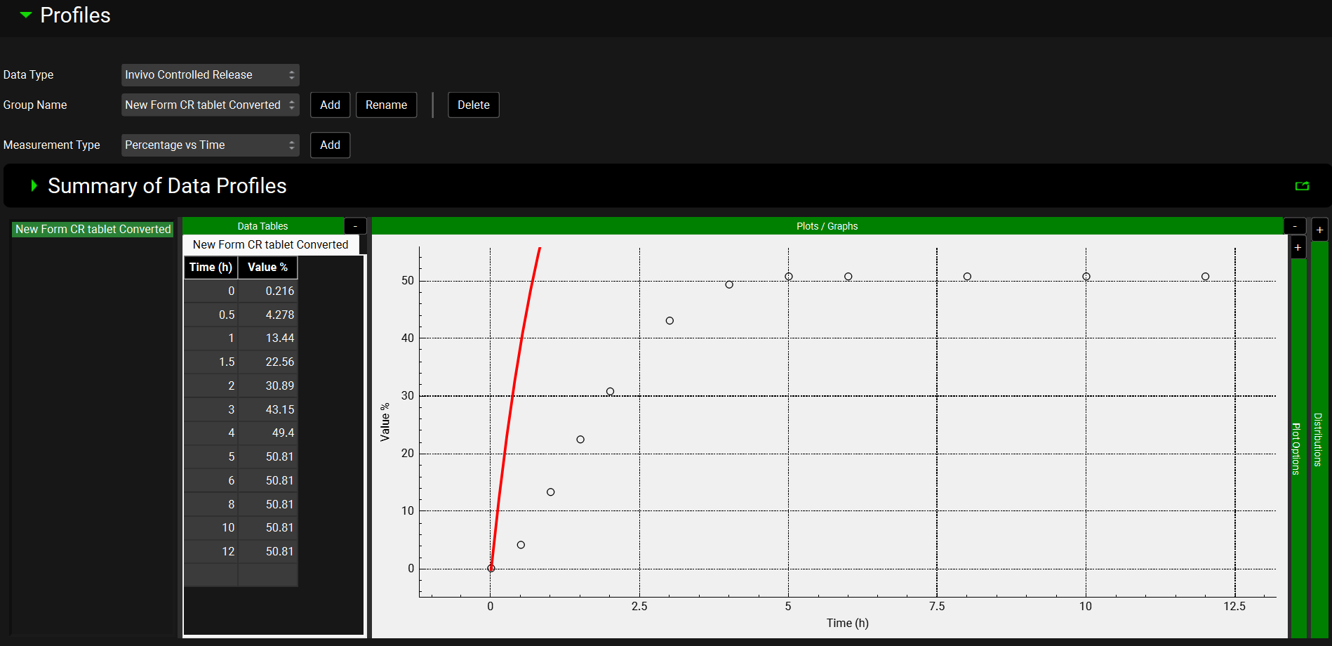
27. Navigate to the Observed Data view and select In Vivo Controlled Release from the Data Type drop-down. The New Form CR tablet Converted profile will be displayed.

28. Go back to the Dosing view. Make sure that the New Form CR tablet formulation is selected. In the Controlled Release sub-panel select In Vivo Controlled Release from the Group Type drop-down.

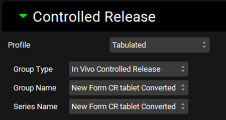
You may need to switch between formulations in the Formulations drop-down for the Group Type to be updated.

29. Navigate to the Simulations view and select New Form CR oral tablet 100mg-2Comps from the Simulations drop-down.

Click on Check Warnings then Run Simulation.

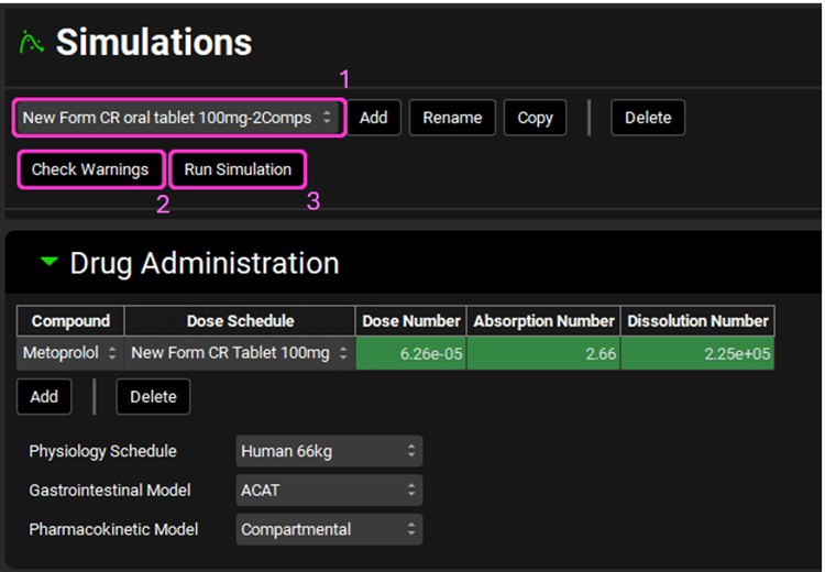
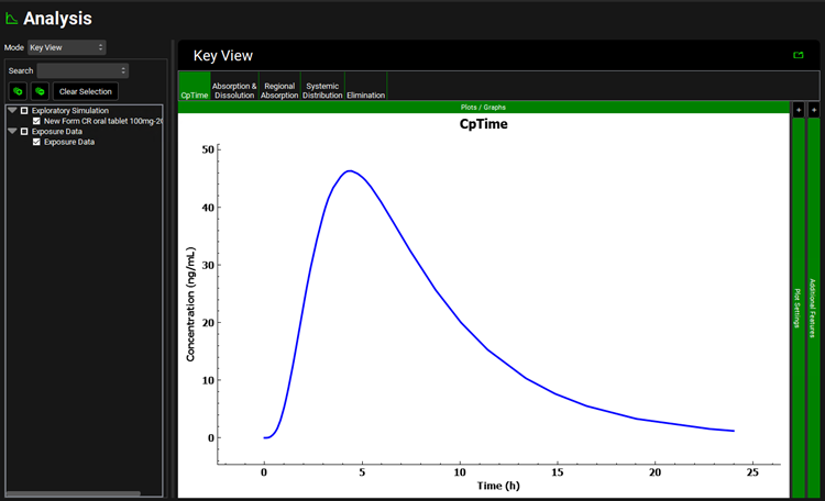
30. After the simulation is run, the view is switched automatically to the Analysis view where the simulated C_p-Time Key View plot is displayed.

This is the expected C_p-Time profile for the New Formulation using the in vivo dissolution profile created from the IVIVC.

31. The saved correlation can also be directly used in the IVIVCPlus™ module without needing to perform convolution and correlation steps.

32. Save the project.

33. Close down GPX™ and reopen the Metoprolol IVIVC project, in the Save Correlation folder, via Select then Browse.

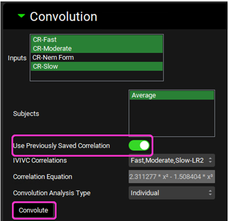
34. Click on IVIVCPlus™ in the Modules pane located on the right-hand side of the interface and scroll down to the Convolution panel.

35. Leave the saved selections in the Inputs and Subjects frames. Click on the Use Previously Saved Correlation toggle. The Fast,Moderate,Slow-LR2 correlation will be shown in the IVIVC Correlations drop-down and the Correlation Equation is displayed below. Click Convolute.

36. When the convolution is finished the observed and predicted plasma concentration-time profiles using the correlation function for all selected inputs will be shown in the left-hand side plot.

The statistics for the fit of the predicted plasma concentration-time profile using the correlation function to the observed data points will be shown in the Statistics for Reconstructed Plasma Concentration Time Profile table. (RSQ=R2, SEP=Standard Error of Prediction, MAE=Mean Absolute Error, and AIC=Akaike Information Criterion).

The Validation Statistics table will show for each input, the Observed and Predicted values and the percent Prediction Error for C_max and AUC_{(0 to t)}.

The C_max and AUC_{(0 to t)} Mean Absolute Prediction Error % are displayed below the table.