Tutorial: P-PSD™ Module
The P-PSD™ Module enables the fitting of a product particle size (the drug substance area available for dissolution in a drug product) to observed in vitro dissolution data for a drug product batch. Using several dissolution profiles obtained in different conditions for a single batch of drug product, the module will recommend which profile to use for fitting and which other profiles to use for model validation. Model prediction performance indicators (Absolute Average Fold Error, and Average Fold Error) are calculated to assess model accuracy and bias. The resulting P-PSD is then transferred to the observed data for use in GastroPlus® for in vivo dissolution prediction of the specific drug product batch.
In this tutorial, we will cover:
Opening the GPX™ project and familiarization with the assets
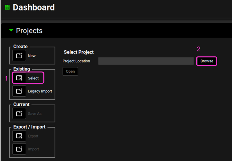
Open GPX™ and, in the Dashboard view, click on the icon next to Select to open an Existing project.
Click Browse and navigate to the C:\Users\<user>\AppData\Local\Simulations Plus, Inc\GastroPlus\10.2\Tutorials\PPSD folder and select the project file PPSD base model.gpproject by clicking on it and clicking Open.
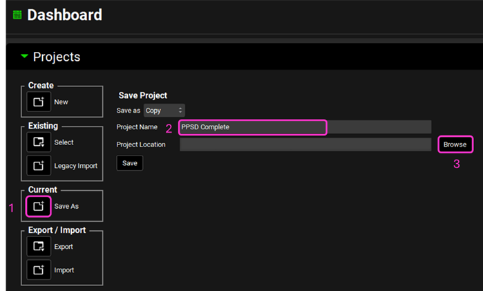
Save a copy of the project by clicking on the icon next to Save As, entering “PPSD complete” as the Project Name and click Browse to navigate to/add a folder to Save the project in. Click Yes on the information window that appears which will also clear the message from the Messages Center indicating that the project has been successfully saved. Note that the name of the project visible in the top right corner of the interface is the one that has just been created.
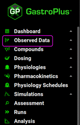
Move through the views on the navigation pane from Observed Data to Simulations, and then Lab Book, observing the information that has been entered in this project.
Loading data from dissolution experiments
Navigate to the Observed Data view.
Select the In Vitro Dissolution Release as the Data Type by clicking in the box containing “Exposure Data” and choosing Invitro Dissolution Release from the drop-down list.
Select “W027180” as the Group Name. This represents the drug product batch number.
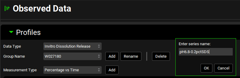
Ensure “Percentage vs Time” is selected as the Measurement Type and click on “Add” to add a series.
Type the series name. This should preferably be a name that describes the dissolution condition. We are going to add data measured in 0.2% SDS at pH6.8 so we can name it “pH6.8-0.2pctSDS”.
You can create as many dissolution experiments linked to the same batch using additional series under the same group. For each series, use a name descriptive of the dissolution experiment.
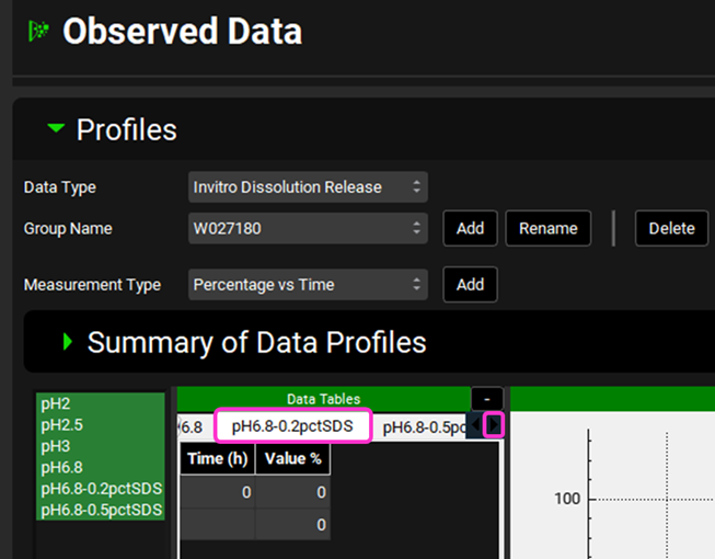
Scroll down to the data tables (if necessary, collapse the Summary of Data Profile table by clicking on the green arrow).
Select the newly added series by clicking on the right-hand arrow to scroll through the series names and click on the pH6.8-0.2pctSDS series name.
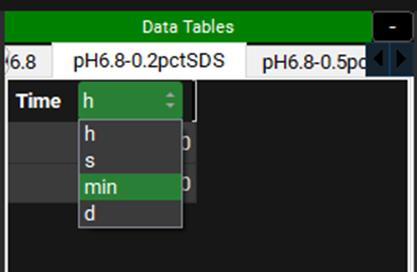
Check that the time units correspond to the raw data you want to input for all the series. Our data is in minutes. To change the units, click on the unit in the column header and select the appropriate one from the list.
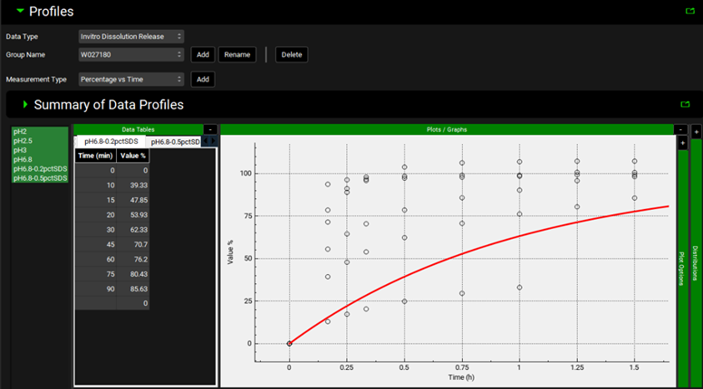
Open the Input Data for PPSD tutorial.xlsx (click the following link to download: Input Data for PPSD tutorial.xlsx) and copy the dissolution data found on the Batch Dissolution data tab (copy both Time and Percent dissolved columns together). Move to GPX™ and paste the data by right clicking in the first cell of the Time column and selecting Paste. The plot should be enabled displaying the observed data. You can identify the newly added series by hovering over the name of the series in the list to the left of the Time column.
Scroll down to below the plot and complete the information for the metadata input using the assay conditions contained in the Input Data for PPSD tutorial.xlsx.
Save your project using the Save button in the right hand corner of the interface and clicking OK on the information message that appears.
Using the P-PSD™ Module
Open the P-PSD™ Module by clicking on P-PSD™ in the Modules pane on the right-hand side of the screen.
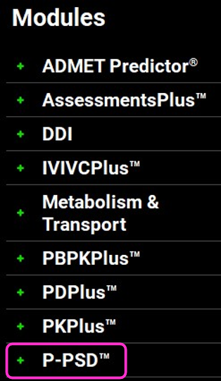
The + signs in the Modules list could appear differently from this screenshot depending on which Modules you license.
Expand the Surfactants panel. This is prepopulated with a list of common surfactants. Details such as the CMC, micelle radius, concentration, and drug affinity to the surfactant are entered in the Inputs Panel since they depend on the medium used for dissolution.
If you need to create your own surfactant, simply click on Add and enter the required details of Surfactant name and Molecular Weight.
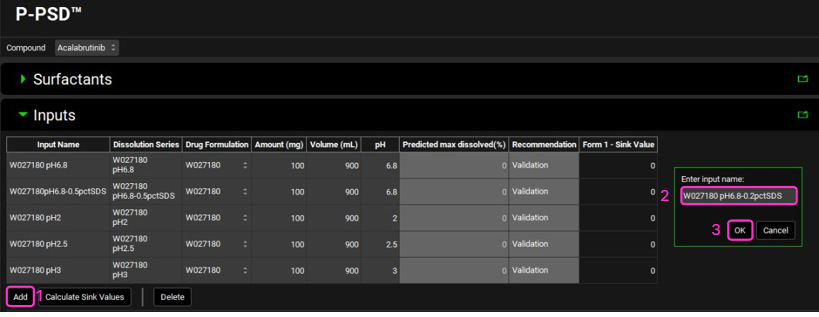
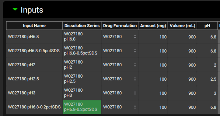
Expand the Inputs Panel and note that a number of inputs relating to the dissolution series added in Observed Data have been prepopulated.
Click on Add to create an Input for the W027180 pH6.8-0.2pctSDS dissolution series we entered in the previous section of this tutorial.
Name the Input using a combination of the drug product batch name and an indication of the dissolution conditions, for this example we will enter “W027180 pH6.8-0.2pctSDS”. Click on OK.
Select W027180 in the Dissolution Series column as the Group Name for the input just created and select pH6.8-0.2pctSDS as the Series Name. This links the input to the correct observed dissolution profile.
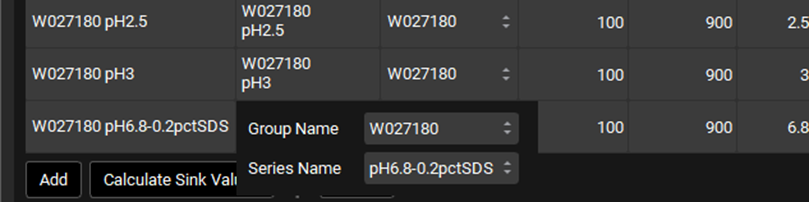
Under the Drug Formulation column, ensure the Drug Formulation “W027180” is selected which corresponds to the batch in question. Confirm the Amount, Volume and pH columns have been populated correctly according to the metadata entered with the Observed Data Series.
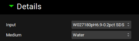
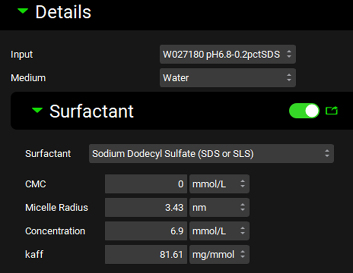
Scroll down and expand the Details panel if necessary. Select the Input just created (W027180 pH6.8-0.2pctSDS) and confirm that the Medium selected is Water.
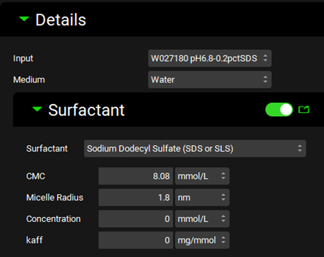
As our dissolution medium contains surfactants select the Surfactant toggle (it will show green if it is activated) and expand the Surfactant panel if necessary.
Select the surfactant “Sodium Dodecyl Sulfate (SDS or SLS)” from the list provided. Some information such as the critical micelle concentration (CMC) and micelle radius are prefilled.
For selected surfactants, an additional Excel tool is provided here ( Size and CMC calculator-v1.0.xlsm) to help you calculate the micelle size and CMC at different temperatures and taking into account the impact of surfactant concentration and counter-ion concentration for ionic surfactants.
For fitting kaff to your measured data an Excel tool is provided here ( Kaff-fitting-tool-v1.0.xlsm).
For more information how to use these tools, please proceed to the next sections of this tutorial (Predicting surfactant CMC and micelle size and Calculating affinity to surfactants).
Predicting surfactant CMC and micelle size
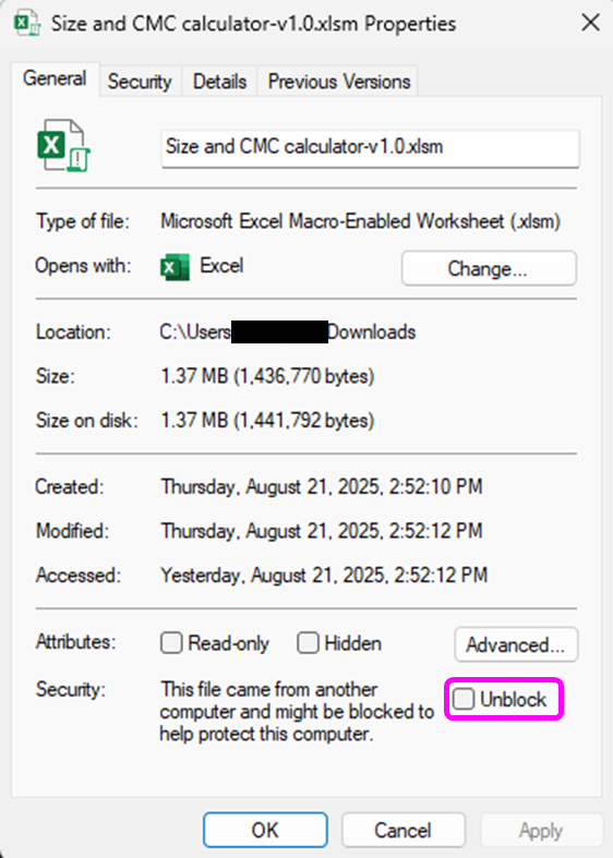
Open the tool: “Size and CMC calculator-v1.0.xlsm” (You can download the file here: Size and CMC calculator-v1.0.xlsm). You may have to first download and enable macros from Excel.
To enable macros in Excel files, right click on the file and select Properties, then check the box next to Unblock under the General tab.
On the Welcome sheet, click on Launch CalcSurf v1.0.
Select the surfactant “SDS or SLS” from the drop-down menu.
Update the temperature, if needed. In this case, the dissolution experiment was conducted at 37°C.
If the surfactant is ionic, you can update the counterion concentration based on the medium composition. For this experiment, the Counterion concentration is 50 mM.
Enter the Surfactant Concentration of 0.2% in the medium to calculate the micelle radius.
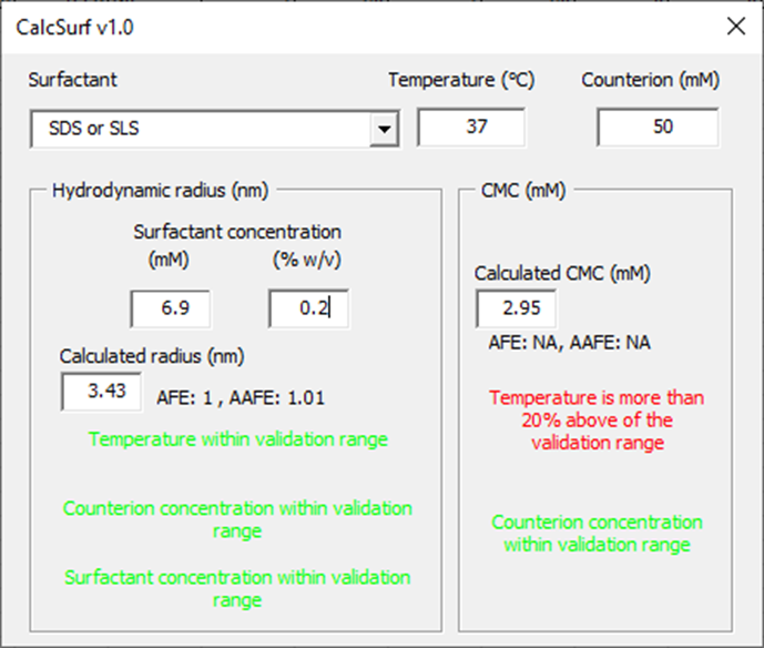
The calculated radius size (nm) and CMC (mM) are provided together with the AFE and AAFE obtained for model validation if all the input parameters are within the validation range. All the messages should be green to indicate that parameters are within the validation range. In this case, the CMC value should be taken with caution as the temperature is outside of the validation range.
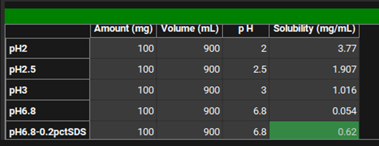
The micelle radius (3.43 nm), surfactant concentration (6.9 mM) and CMC (2.95 mM) can now be copied to the appropriate cells in the Surfactant panel. However, the observed data should also be considered – review the effect of SDS on the apparent solubility which can be found in the Physchem Properties tab in the Input Data for PPSD tutorial.xlsx (click here to download: Input Data for PPSD tutorial.xlsx). Here it can be seen that at the lowest SDS concentration there is an increase in apparent drug solubility and therefore, the CMC should actually be set to 0.
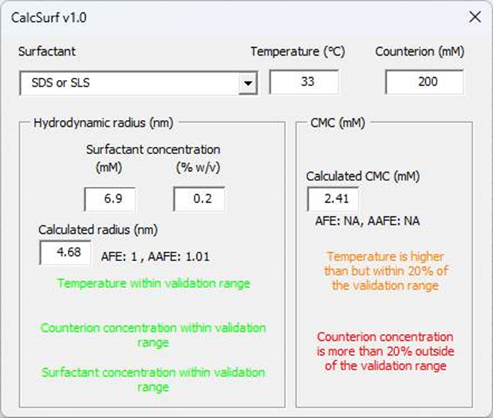
If one of the input parameters is outside of the validation range for the model, the AFE and AAFE are not shown and a colored warning message will indicate how far the input parameter is outside of the range. In the example below, the temperature is lower but within 20% of the validation range and the counterion concentration more than 20% outside of the validation range.
Calculating affinity to surfactants
Open the tool: “Kaff-fitting-tool-v1.0.xlsm” (click here to download: Kaff-fitting-tool-v1.0.xlsm).
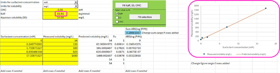
Indicate the units of your data. It is recommended to use mM for surfactant concentration and mg/L for solubility, and these are the units required for this example. Type best guess values for CMC (0, defined in the previous section), Kaff (1) and aqueous solubility (S0; 54 mg/L from the solubility data generated in the relevant media without surfactant, see step 3 below).
Input your measured drug solubility (Column B from line 11) versus surfactant concentration (Column A from line 11) which can be found in the Physchem Properties tab in the Input Data for PPSD tutorial.xlsx. Clear the additional entries from rows 16 and 17 in columns A, B, and E.
You can either fit the three parameters S0, Kaff, and CMC by clicking on Fit Kaff, S0, CMC. Alternatively, you can tick only the parameters that you want to fit and click on Fit selection. In this case we are only going to fit Kaff so check the box next to Kaff. Click “Fit Selection”.
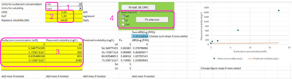
The results of the fit are graphically shown to the right.
The affinity to the surfactant Kaff in mg/mmol can be used directly in the P-PSD™ Module.
P-PSD™ in GPX™
Update the information about the CMC, Micelle Radius, Concentration of surfactant in the medium and affinity of the drug substance with the micelle determined in Predicting surfactant CMC and micelle size and Calculating affinity to surfactants, ensuring the correct input is selected at the top of the Details panel.
Notice the input boxes for entering amount of the drug in the dosage form (Assay (percentage of target)). In this case the batch analysis indicated that the tablet was 100% of the target.
Notice the input boxes for the drug product disintegration or opening time in vitro and the degradation rate of the drug in the dissolution medium. Neither are applicable for this example.
Indicate the drug aqueous surface solubility in the dissolution medium, which can be found in the Physchem Properties tab in the Input Data for PPSD tutorial.xlsx. At pH6.8 it is estimated to be 54 mg/L. Once the Aqueous Surface Solubility is entered, the Fu is calculated.
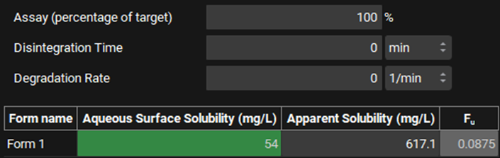
At least one aqueous surface solubility is needed for dissolution in media without surfactant. Once the aqueous surface solubility is entered the fraction of drug unbound is calculated if micelles are present.
Save your project using the Save button in the right hand corner of the interface and clicking OK on the information message that appears.
Once all the details for each dissolution experiment have been entered under the Details view (in this example these have been pre-populated for the other experiments), scroll back up to the Inputs view and click on Calculate Sink Values. Based on the details entered, the sink value and the predicted maximal percentage dissolved are calculated.
The P-PSD™ module recommends the experiment to use for P-PSD fitting (Optimization) and the ones for model validation.
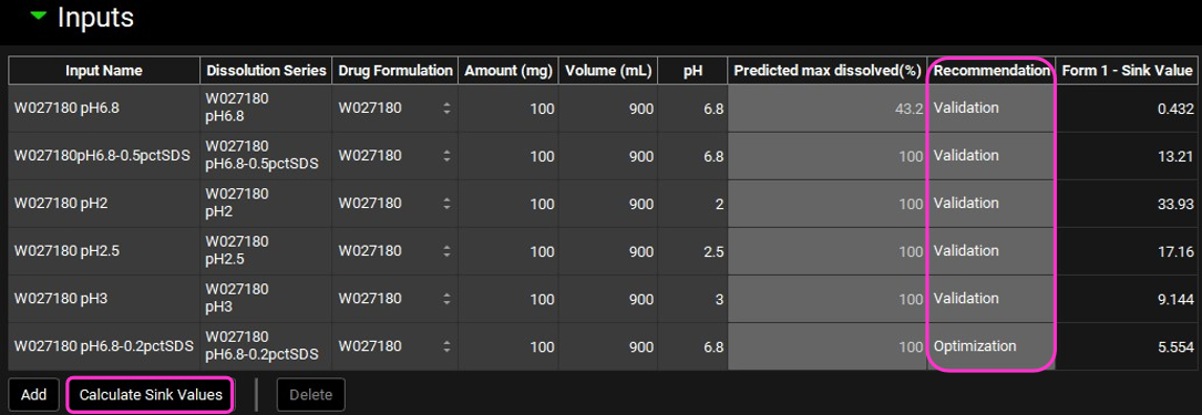
If you keep adding dissolution inputs after you have clicked on Calculate Sink Values, click again on this button since recommendations for input experiment for P-PSD fitting and validation may have changed.
Fitting the P-PSD
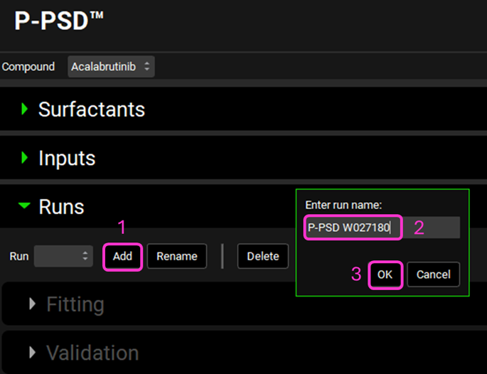
Expand the Runs View and click on Add run.
Call your run, “P-PSD W027180” and click OK.
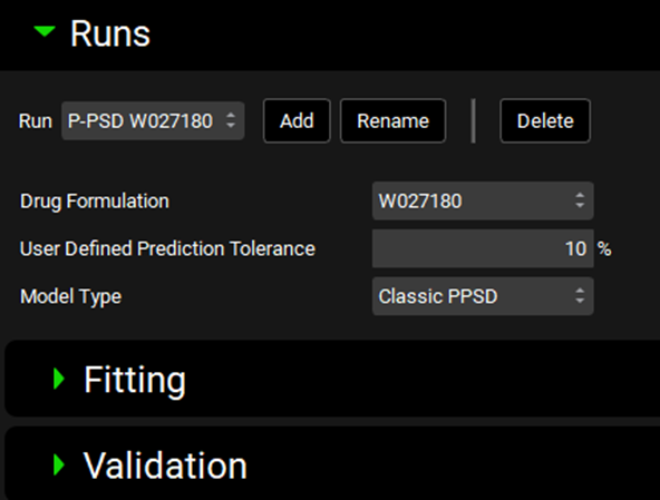
Ensure the drug formulation “W027180” is selected and define the User Defined Prediction Tolerance (percent error) for the fitting. It is recommended to leave the default of 10% for the first iteration then reduce the tolerance to improve the fitting if needed.
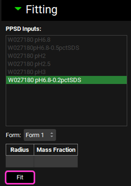
Expand the Fitting subpanel and select the dissolution data input(s) which will be used for fitting by clicking on it, in this case, W027180 pH6.8-0.2pctSDS was recommended by the program.
You have different options for fitting. Either you let the P-PSD™ Module find the least number of bins and mass distribution that matches your dissolution, or you can add your own starting points for bin size and mass distribution by updating the radius and mass fraction information of the P-PSD. In this example we will let the module find the solution, so click on Fit.
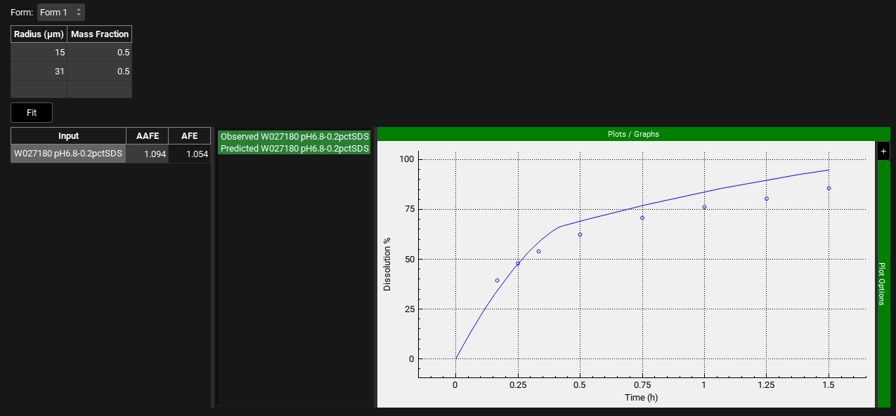
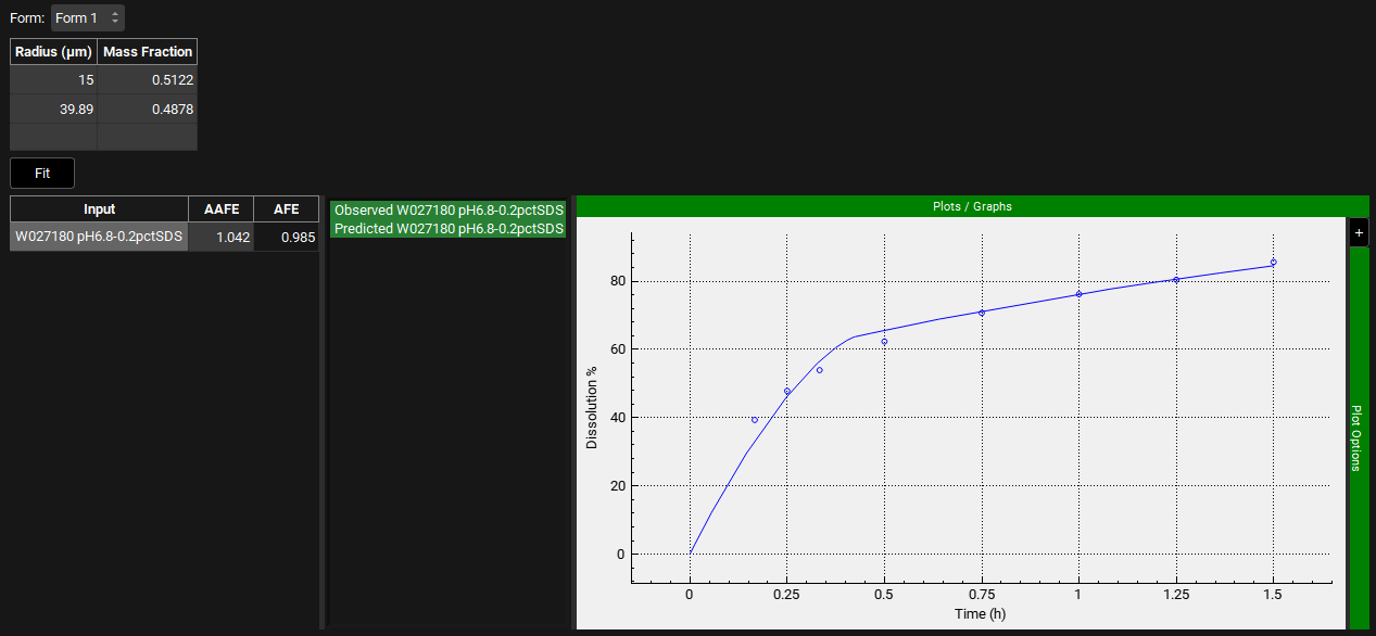
The P-PSD which best fits the dissolution data input(s) you have selected will be displayed and beneath that the observed and predicted dissolution data are plotted. Press the Ctrl key and click on the name of each series to the left of the plot update the plot. The AAFE and AFE are also displayed next to the dissolution data.
You can decide to reduce the predefined tolerance to improve fitting. Note that if you reduce the tolerance too much, the following message may show if the P-PSD™ Module could not find a particle size distribution that could match your input data within the tolerance.

Although the fit is reasonable, there is a slight overprediction in the initial phase. Reduce the User Defined Prediction Tolerance to 5% and click on Fit again. Press the Ctrl key and click on the name of each series to the left of the plot update the plot. The AAFE and AFE have both improved and the shape of the dissolution profile is well captured.
Once you are satisfied with the P-PSD fit, you can move to Validation.
Validate and Transfer the P-PSD
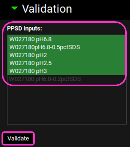
Scroll down and expand the Validation view.
Select the dissolution data inputs you want to use for model validation by clicking on each in turn or clicking on the first one and dragging to the final one you wish to select – it is recommended to select all dissolution profiles with the exception of the one used for fitting.
Click on Validate.
The predictions and observations will be shown. Press the Ctrl key and click on the name of each series to the left of the plot update the plot.
The AAFE and AFE for all the dissolution predictions are shown on the left of the dissolution curves.
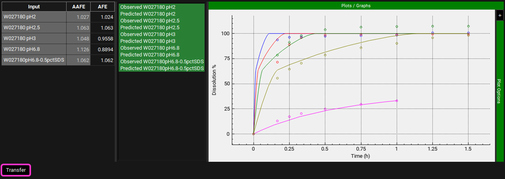
Whilst the initial rate of dissolution of the pH2 and pH2.5 profiles is overpredicted, these are capsule dose forms and potentially require a degradation time to account for the capsule opening time. The AAFE and AFE for each profile are within 13% and therefore is deemed acceptable. Therefore, the validation of the P-PSD is satisfactory so we can scroll down and click on Transfer.
A message will confirm that the transfer is complete. Click on OK or press Enter on the message.
Navigate to the Observed Data View and select the Particle Size Distribution Data Type.
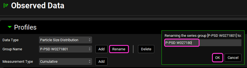
The transferred P-PSD appears under the Group name using the P-PSD™ Module Run name with the added number 1 for the first export. If you refine the P-PSD fit for the same run and click again on export, the group name will have the run name and number 2. You can rename this group by clicking on Rename, deleting the 1, and clicking OK.
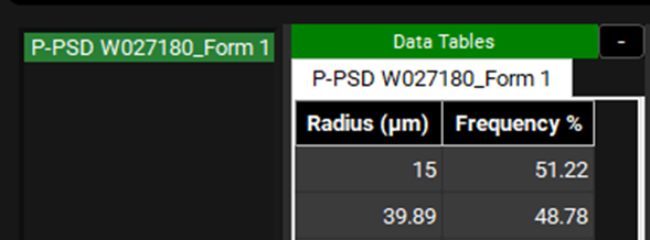
The transferred P-PSD can be seen as the frequency distribution of particle size with a unique mass distribution and can be used for predicting in vivo dissolution of the batch in question.
Save your project using the Save button in the right hand corner of the interface and click OK on the information message that appears.
Using the P-PSD for in vivo dissolution predictions
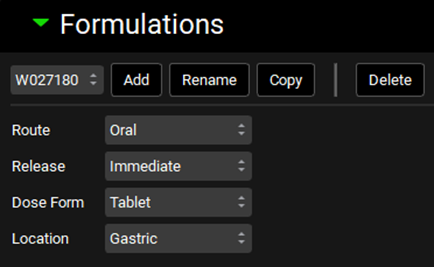
Under the Dosing view, expand the Formulations panel and ensure that the Formulation “W027180” for which in vivo dissolution should be predicted using the P-PSD is selected.
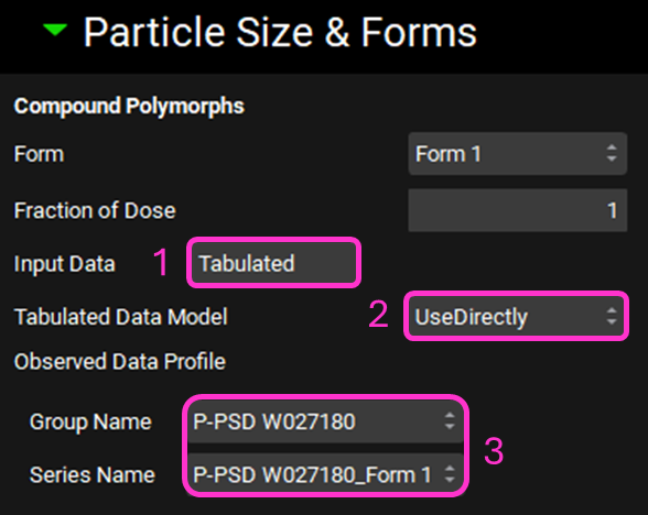
Expand the Particle Size & Forms subpanel. Select “Tabulated” for Input Data by clicking in the box that says Distribution.
Ensure “UseDirectly” is selected for Tabulated Data Model.
Confirm that the Observed Data group created by the transfer of the P-PSD output is selected: Group Name: P-PSD W027180; Series Name: P-PSD W027180_Form 1.
Navigate to the Simulations view and ensure the simulation “W027180 100mg PO tablet” is selected.
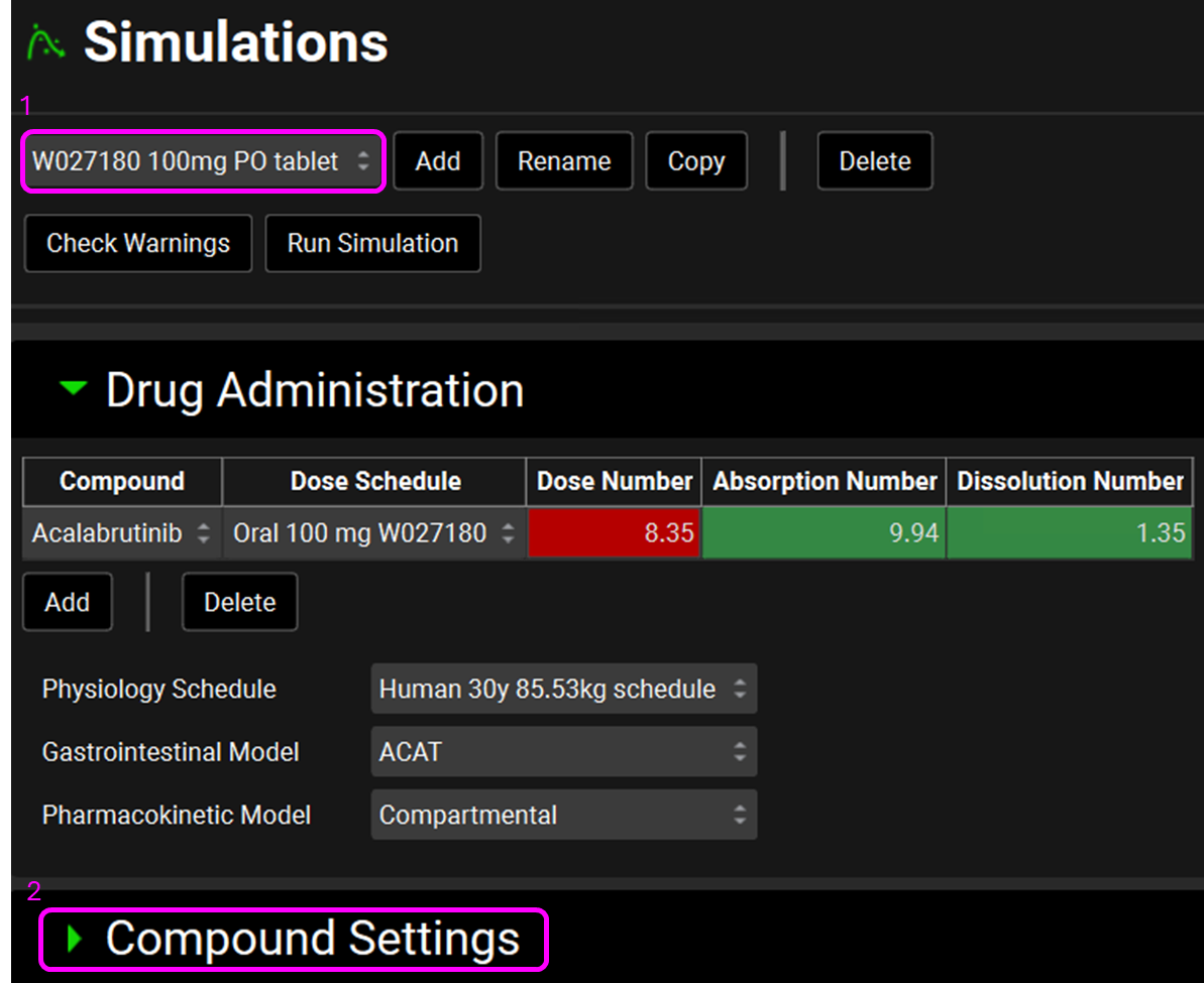
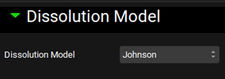
Expand the Compound Settings panel, move to the Dissolution Model subpanel, expand it and confirm that the Johnson model is selected (this is a pre-requisite to enable the P-PSD to be used as an input in the simulation).
Save your project using the Save button in the right hand corner of the interface and click OK on the information message that appears.
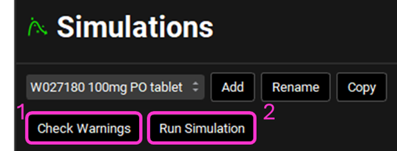
Click Check Warnings (underneath the Simulation name at the top of the view) and then Run Simulation.
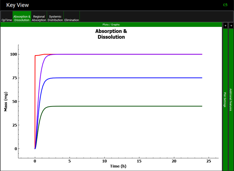
When the program automatically switches to the Analysis view, click on the Absorption & Dissolution plot and notice the shape of the red Total Dissolved curve is driven by the P-PSD.