Indirect Response PD Models

Unlike the direct response PD model, an indirect response PD model accounts for lag time in the observed PD effect as well as for hysteresis, which occurs when the same concentration of drug in plasma produces two different levels of the PD effect, depending on the time course of the plasma concentration. Five types of indirect response PD models are available in GastroPlus®. See:

Effect Compartment model

Figure 3-5: Effect Compartment model schematic (indirect link)

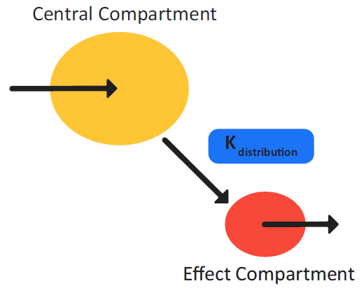
Figure 3-5 is a schematic of the Effect Compartment model. The Effect Compartment model assumes that the delay in the pharmacological action of the drug from the time that it enters the plasma compartment is due to the re-distribution of the drug to the effect compartment, which is the true site of the pharmacological action. Equation 3-7 shows the transfer rate of the drug between the two compartments.

Equation 3-7: Drug transfer rate for the Effect Compartment model

where:

Variable	Definition
	The amount of drug in the plasma compartment.
	The amount of drug in the effect compartment.
	The drug transfer rate constant from the plasma compartment to the effect compartment.
	The drug transfer rate constant from the effect compartment to the plasma compartment.

Equation 3-8 describes the Effect Compartment model in terms of distribution of the drug.

Equation 3-8: Drug mass in the Effect Compartment model

where:

Variable	Definition
	The rate of distribution of drug from the plasma compartment to the effect compartment, referred to as the inter-compartmental distribution rate.
	The total or unbound concentration of drug in the plasma compartment.
	The total or unbound concentration of drug in the effect compartment.

The concentration of the drug in the Effect Compartment model is then linked to either the Emax model or the Sigmoid Emax model as described in Direct Response PD Models.

Class I – Class IV models

Dayneka ¹ proposed a set of indirect response models that explained the lag time of the PD effect and the apparent lack of direct correlation of with C_p by means of mechanistic equations that related the C_p on the stimulation or inhibition of the generation or dissipation of the effect, where if the rate of generation and dissipation of the PD effect variable (E) in the absence of drug can be described by zero and the first-order rate constants k_in and k_out, respectively, then Equation 3-9 gives the rate of change of the effect variable in the absence of drug.

Equation 3-9: Rate of change of PD effect variable in the absence of drug

Under steady state conditions, k_in = k_outR₀, where R₀ is the baseline PD effect.

You can combine any of these four models with the effect compartment model to simulate indirect effect that is linked to a hypothetical effect compartment. See:

Class I and Class II indirect response models (inhibitory)

Class III and Class IV indirect response models (stimulatory)

Class I and Class II indirect response models (inhibitory)

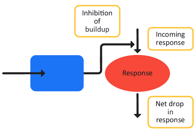
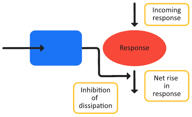
Class I and Class II indirect response models follow the standard inhibitory equation (Equation 3-10), where Class I models represent inhibitory processes that operate on the generation of the PD effect variables and Class II models represent the inhibitory processes that operate on the dissipation of the PD effect variables.

Equation 3-10: Standard inhibitory equation

Figure 3-6 is a schematic of a Class I indirect response model and Equation 3-11 shows the changes in the effect variable over time for the model.

Figure 3-6: Indirect response model, Class I

Equation 3-11: Change in PD effect variable over time, Class I indirect response model

Figure 3-7 is a schematic of a Class II indirect response model and Equation 3-12 shows the changes in the effect variable over time for the model.

Figure 3-7: Indirect response model, Class II

Equation 3-12: Change in PD effect variable over time, Class II indirect response model

For both Class I and Class II models, you must estimate the following parameters: k_in, k_out, I_max, and IC₅₀.

Class III and Class IV indirect response models (stimulatory)

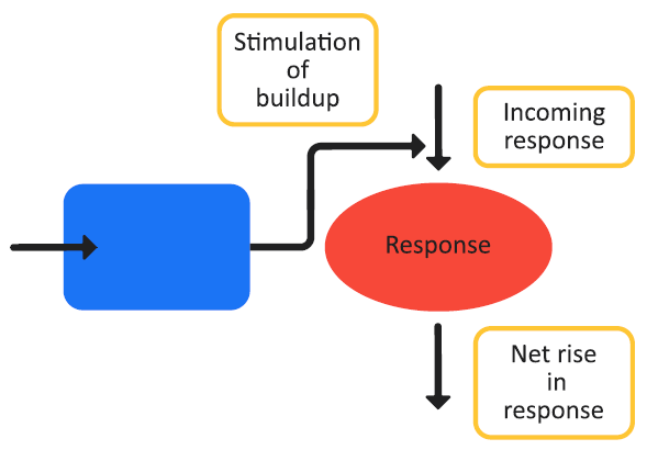
Class III and Class IV indirect response models follow the standard stimulatory equation (Equation 3-13), where Class III models represent the stimulation processes that operate on the generation of the PD effect variables and Class IV models represent the stimulation processes that operate on the dissipation of the PD effect variables.

Equation 3-13: Standard stimulatory equation

Figure 3-8 is a schematic of a Class III indirect response model and Equation 3-14 shows the changes in the effect variable over time for the model.

Figure 3-8: Indirect response model, Class III

Equation 3-14: Change in PD effect variable over time, Class III indirect response model

Figure 3-9 is a schematic of a Class IV indirect response model and Equation 3-14 shows the changes in the effect variable over time for the model.

Figure 3-9: Indirect response model, Class IV

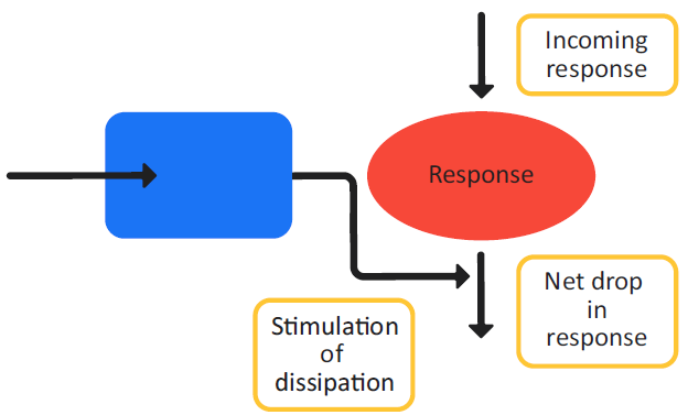
Equation 3-15: Change in PD effect variable over time, Class IV indirect response model

For both Class III and Class IV models, you must estimate the following parameters: k_in, k_out, E_max, and EC₅₀.

Cell killing model: Phase non-specific

The basic pharmacodynamics model for cell proliferation and phase non-specific killing was presented by Jusko ² and it includes the irreversible reaction between the drugs in the effect compartment and the target cells. For this model, the drug concentration in the effect compartment (C_e), which is the true site of the pharmacological reaction, can be calculated according to Equation 3-8. The rate of change in quantity of the target cells (the PD effect) is shown in Equation 3-16.

Equation 3-16: Rate of change in quantity of target cells (Cell killing model, phase non-specific)

where:

Variable	Definition
	The cell growth rate constant, which is the difference between the natural mitotic rate and physiologic degradation.
	The rate of the irreversible reaction.

Bacteria killing and growth (BKG) model

Kristoffersson ³ presented the pharmacodynamics model for bacteria killing and growth. As shown in Figure 3-10, the model consists of two bacterial populations: one antibiotic susceptible population (sub-population 1, which is the main population) and one pre-existing antibiotic resistant population (sub-population 2).

Figure 3-10: Bacteria killing and growth model schematic

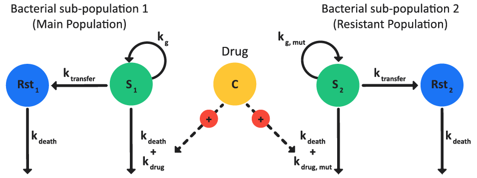
In each sub-population, the bacteria exist in two states:

Proliferating, antibiotic-susceptible (S) bacteria.

Resting (Rst), non-proliferating, antibiotic-resistant bacteria.

The initial state of the system is defined by the total number of bacteria that are in the resistant sub-population (S2 + R2) and the total number of bacteria that are in the resting state in each sub-population as shown in Equation 3-17 (an equation set).

Equation 3-17: Initial state of the system, BKG model

where:

Variable	Definition
	The initial number of bacteria.
	The percent of pre-existing antibiotic-resistant bacteria.
	The percent of bacterial cells that are in the resting state.
	Resting state of sub-population 1.
	Resting state of sub-population 2.

Equation 3-18 (an equation set) defines the transfer rate from the S population to the R population.

Equation 3-18: Transfer rate from S population to R population, BKG model

where:

Variable	Definition
	The maximum number of bacteria in the stationary phase.
	The growth rate constant for antibiotic-susceptible bacteria.
	The rate constant for bacterial natural death.
	The total number of bacteria across all sub-populations.

Equation 3-19 (an equation set) describes the effect of the drug on each bacterial sub- population, where the effect is a function of the drug concentration.

Equation 3-19: Effect of the drug on each bacterial sub-population, BKG model

where k_drug,mut is the growth rate constant for pre-existing antibiotic-resistant bacteria.

Equation 3-20 (an equation set) describes how to apply these functions to study the effect of the drug using either a Power model or a Sigmoidal model, respectively.

Equation 3-20: Effect of an antibiotic drug with Power model or Sigmoidal model

where:

Variable	Definition
	The drug concentration.
	The Hill factor in the drug-effect relationship.
	The maximum kill rate constant.
	The concentration of the drug that produces 50% of E_max.
	The shift in the concentration of the drug that is required for the drug to have the same effect on the mutant bacteria as it does on the antibiotic-susceptible bacteria,

Precursor dependent models (Class V – VIII)

The basic indirect response models (Class I–IV) can be extended to incorporate a precursor compartment to describe the development of tolerance and rebound of the pharmacodynamics response due to the depletion or accumulation of a physiological precursor that is responsible for generating drug effects ⁴ ⁵ . Figure 3-11 is a schematic of a precursor-dependent indirect model and Equation 3-21 (an equation set) shows the model calculations.

Figure 3-11: Precursor-dependent indirect response model

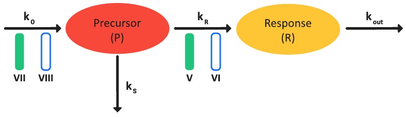
Equation 3-21: Calculations for a precursor-dependent indirect response model

where:

Variable	Definition
	The amount of precursor.
	The zero order rate constant for precursor production.
	The first order rate constant for response production.
	The first order rate constant for loss of precursor.
	The first order rate constant for loss of response.
	The inhibition (Class VII) or stimulation (Class VIII) of precursor production.
	The inhibition (Class V) or stimulation (Class VI) of response production.

To incorporate a circadian rhythm in the baseline response, the k_R can be characterized as a cosine function as shown in Equation 3-22.

Equation 3-22: Incorporating a circadian rhythm in the baseline response, precursor-dependent indirect response model

where:

Variable	Definition
	The mean production of response rate.
	The amplitude of rate.
	The time of occurrence of the peak production rate.

Dayneka, N.L., Garg, V., et al. (1993). “Comparison of four basic models of indirect pharmacodynamic responses.” J. Pharmacokinet. Biopharm. 21(4): 457-78.
Jusko, W.J. (1971). “Pharmacodynamics of chemotherapeutic effects: dose-time- response relationships for phase-nonspecific agents.” J. Pharm. Sci. 60(6): 892-5.
Kristoffersson, A.N., David-Pierson, P., et al. (2016). “Simulation-Based Evaluation of PK/PD Indices for Meropenem Across Patient Groups and Experimental Designs.” Pharm. Res. 33(5): 1115-1125.
Felmlee, M.A., Morris, M.E., et al. (2012). “Mechanism-based pharmacodynamic modeling.” Methods Mol. Biol. 929: 583-600.
Sharma, A., Ebling, W.F., et al. (1998). “Precursor-dependent indirect pharmacodynamic response model for tolerance and rebound phenomena.” J. Pharm. Sci. 87(12): 1577-84.