Tutorial: Metabolism & Transport Module

Metabolism and Transporter module

The Metabolism and Transporter Module is an optional module that extends the capabilities of GastroPlus® to simulate saturable gut and liver metabolism, and saturable carrier-mediated transport by both influx and efflux proteins in the gut. When used in PBPK models, it also enables simulating saturable enzymatic metabolism and saturable influx and efflux transport in all PBPK tissue compartments.

In this tutorial, we will cover:

• Using in vitro clearance data

• Metabolite Tracking

• Transporter-based IVIVE - Metabolism and Transporter module

Using in vitro clearance data

The following example illustrates the use of the Metabolism and Transporter Module using midazolam as the test drug.

Midazolam is completely absorbed from the GI tract but has a bioavailability in the order of 25-30% because of high first pass extraction in the gut and in the liver. CYP3A4 enzymes in the gut and the liver are responsible for the biotransformation of midazolam. The amount of active CYP3A4 in the gut can be reduced by ingestion of grapefruit juice (GFJ). Based on in vitro incubation with liver microsomes, the in vitro enzyme kinetic constants of biotransformation V_max and K_m have been measured and reported in the literature ¹ .

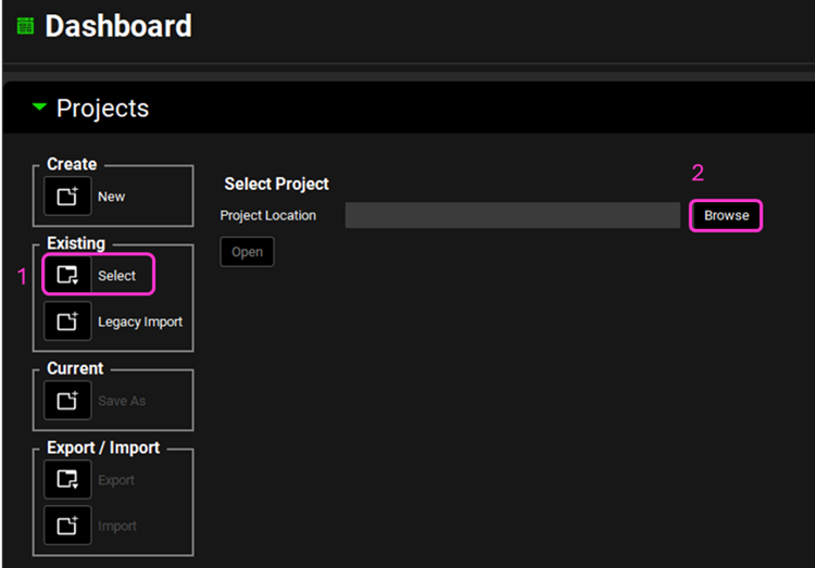
1. Open GPX™ and, in the Dashboard view, click on the icon next to Select to open an Existing project.

2. Click Browse and navigate to the C:\Users\<user>\AppData\Local\Simulations Plus, Inc\GastroPlus\10.2\Tutorials\M&T-Midazolam and select the project file Midazolam.gpproject by clicking on it and clicking Open.

There are two compounds in this project: Midazolam AP10.4 and Midazolam.

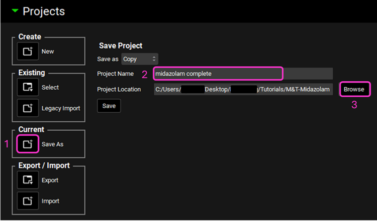
3. Save a copy of the project by clicking on the icon next to Save As, entering “Midazolam complete” as the Project Name and click Browse to navigate to/add a folder to Save the project in. Click Save - you will see an information message in the Messages Center indicating that the project has been successfully copied. This message will disappear once you click 'Yes' on the pop-up window that also appears. Note that the name of the project visible in the top right corner of the interface is the one that has just been created.

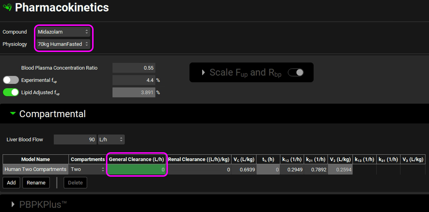
4. Navigate to the Pharmacokinetics view and select Midazolam from the Compound drop-down. Expand the Compartmental panel by double clicking the panel header or clicking on the green arrow. Examine the compartmental PK parameters - the 2-compartment model was fitted to an IV data for Midazolam. Set the General Clearance entry to zero. The linear clearance will not be used, because we will use in vitro data from microsomes in a nonlinear metabolism model to calculate concentration-dependent clearance.

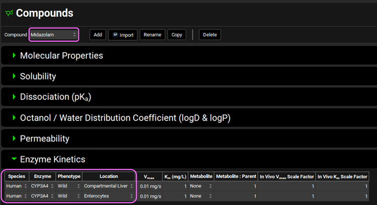
5. Navigate to the Compounds view and make sure Midazolam is selected from the Compound drop-down. Expand the Enzyme Kinetics panel by double clicking the panel header or clicking on the green arrow. We will now add two enzyme entries to the table. Click Add (found under the Enzyme Kinetics table) and after the first entry has been created click Add again.

Leave Human as the selected Species. From the Enzyme drop-down, ensure CYP3A4 is selected and select Enterocytes from the Location drop-down. For the second row, select CYP3A4 from the Enzyme drop-down and ensure Compartmental Liver is selected for the Location. Leave the Wild Phenotype selected for both rows.

6. Save the Project by clicking on “Save” in the top right corner of the interface and then click “OK” on the Save completed message.

The reported K_m and V_max values will be converted to in vivo conditions and units for GastroPlus® using the Metabolism & Transport module.

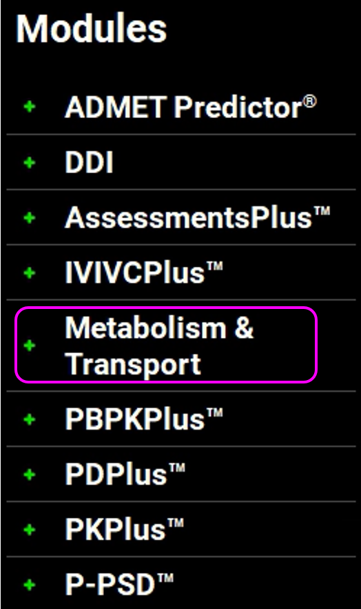
7. Click on Metabolism & Transport in the Modules pane on the right-hand side of the interface.

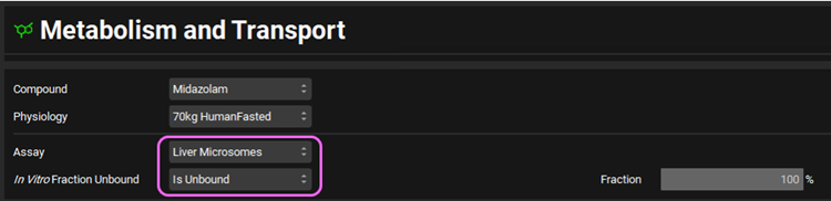
8. Make sure that Midazolam is selected from the Compound drop-down. Since there is only one physiology in this project, 70kg HumanFasted will be automatically selected from the Physiology drop-down. Select Liver Microsomes from the Assay drop-down and Is Unbound from the In Vitro Fraction Unbound drop-down.

9. Expand the Scaling Factors panel to see the default entries. We will use all default parameters.

If the In Vitro Microsomal Protein Concentration box appears empty, you can either click on the Restore Defaults button (as the default value is used in this tutorial) or you can either type directly the value in the box.

10. Expand the Metabolism panel. You will notice that there will be an entry for CYP3A4 in the Enzyme-Specific table.

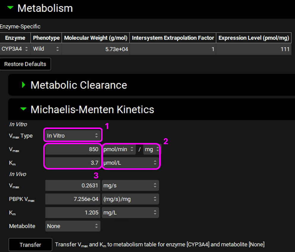
11. Expand the Michaelis-Menten Kinetics sub-panel. The reported ¹ in vitro kinetic constants obtained from liver microsomal incubations of Midazolam are: V_max = 850 pmol/min/mg protein and unbound K_m = 3.7 μmol/L.

12. Select In Vitro from the V_max Type drop-down if not already selected. Choose the appropriate units and then enter the in vitro V_max and K_m. The converted in vivo V_max and K_m should be 0.2631 mg/s and 1.205 mg/L, respectively.

13. Click Transfer (Transfer V_max and K_m to metabolism table for enzyme [CYP3A4] with metabolite [None]). An information message will appear in the Messages center letting you know that the V_max and K_m have been transferred to the Enzyme Kinetics panel in the Compounds view. Click Done to Clear the message.

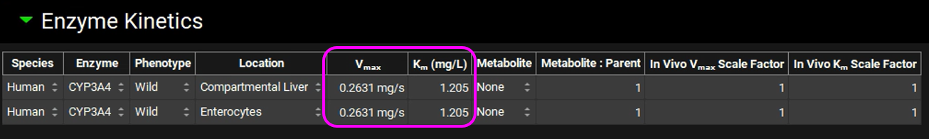
14. Navigate to the Compounds view and notice how the in vivo V_max and K_m have been transferred.

15. Save the project and click OK.

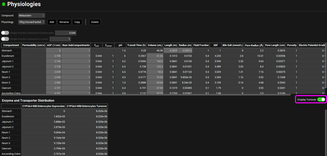
16. Navigate to the Physiologies view and expand the Gastrointestinal panel. Scroll down to the Enzyme and Transporter Distribution table at the bottom of the panel. Examine the CYP3A4 Wild Enterocytes Expression. These numbers were automatically loaded because one of the Enzyme Kinetics entries in the Compounds view shows the enzyme name CYP3A4 with the location as Enterocytes. These are the relative amounts of CYP3A4 in each GI compartment to the amount of CYP3A4 in the liver and are used to scale the rate of drug metabolism in the gut based on the rate in the liver.

Select the Display Turnover toggle on the right-hand side of the panel. A column will be added showing the CYP3A4 Wild Enterocytes Turnover rates for the enzyme in each GI compartment. These are used in drug-drug interaction predictions for time-dependent inhibitors.

17. Navigate to the Simulations view. There is one simulation already created in this project (Midazolam15mg NoGFJ). Expand the Drug Administration panel and see how Midazolam is selected from the Compound drop-down.

Note – NoGFJ represents dosing in the absence of Grapefruit Juice.

18. Expand the Compound Settings panel and make sure the Metabolism toggle is on.

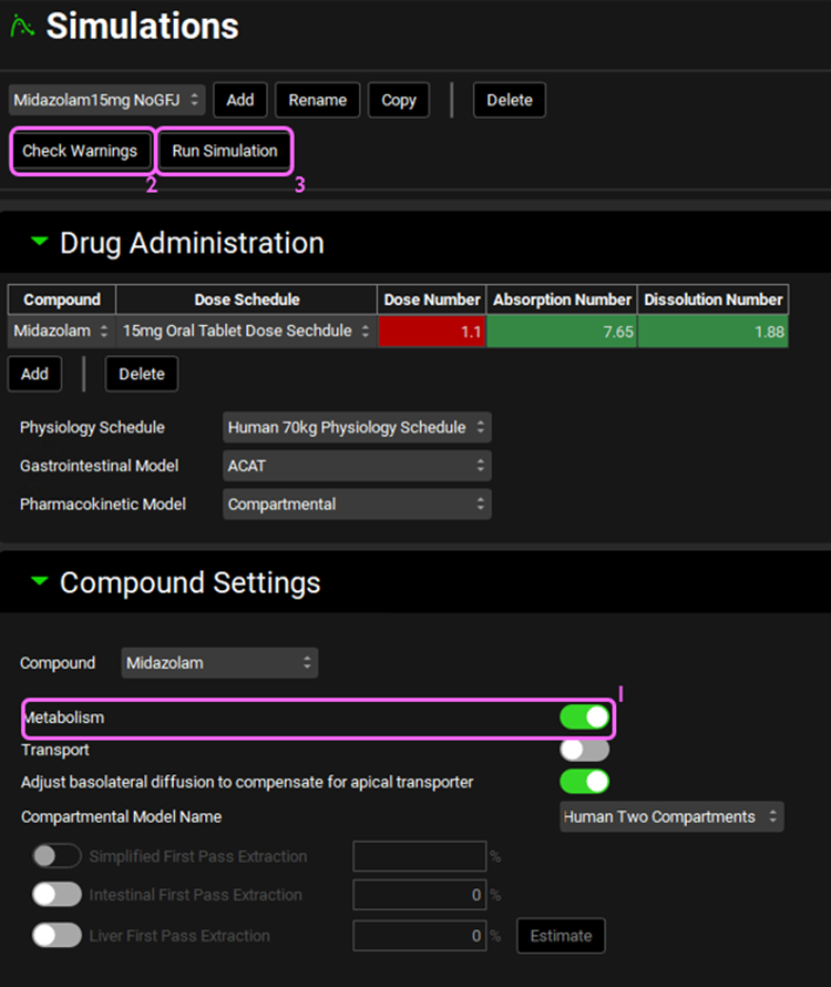
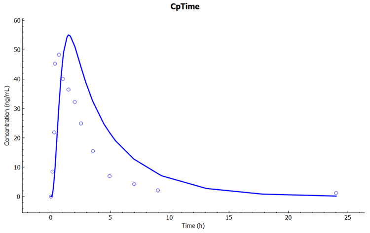
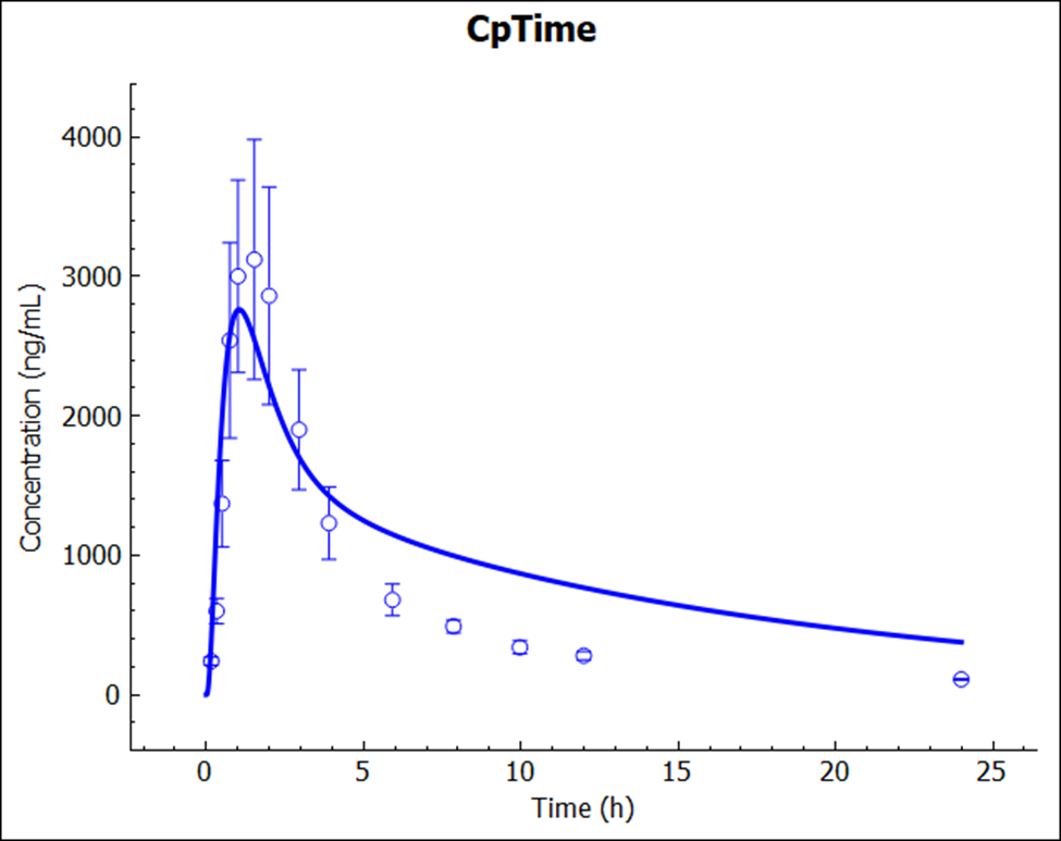
19. Click on Check Warnings at the top of the Simulations view and then Run Simulation. Once the simulation finishes, the program switches automatically to the Analysis view. The C_p-Time plot will be displayed in Key View mode.

20. Examine the predicted and observed C_p-Time. Notice that the simulation is a very good estimate of the actual human C_p-Time. Remember that this is not a fitted model – clearance was calculated from in vitro measurements of metabolism in microsomes. The only fitted parameters were the PK parameters for distribution (V_c, K12, and K21) from a single IV dose of Midazolam. If you had used PBPKPlus™ to model this drug with physiologically based pharmacokinetics, you would have predicted human C_p-Time this close with no human or animal data at all!

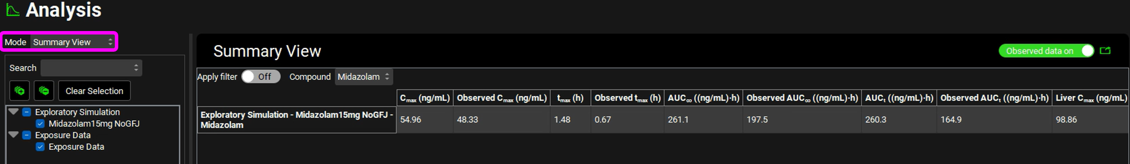
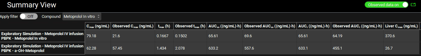
21. Switch the Analysis Mode from Key View to Summary View and compare the Observed and Calculated C_max, T_max, and AUC values (scroll the table right to see other parameters).

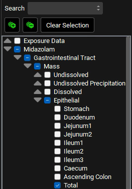
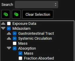
22. Switch the Analysis Mode from Summary View to Deep View. Under the Deep View panel, expand Midazolam in the series list tree by clicking on the grey arrow. Select the following series from the list by clicking in the checkbox next to the series name:

a. Midazolam->Gastrointestinal Tract->Mass->Epithelial->Total

b. Midazolam->Systemic Circulation-> Mass->Liver

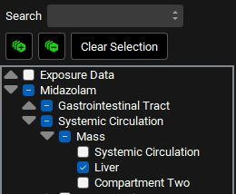
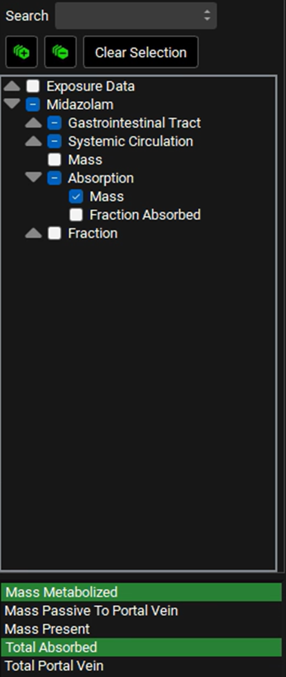
c. Midazolam->Absorption->Mass

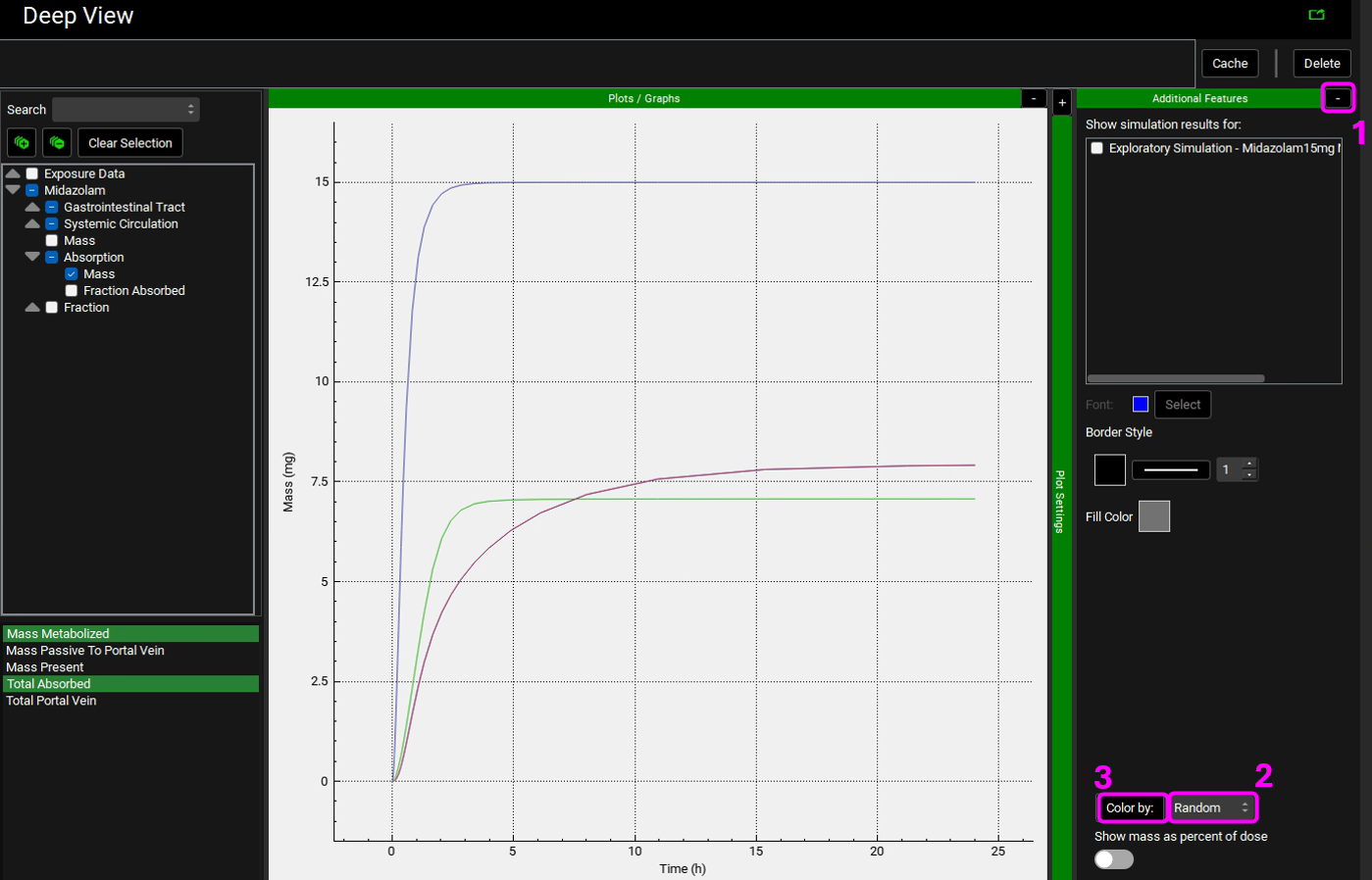
In the variables list at the bottom, select Mass Metabolized by clicking on it, and then hold down CTRL and click on Total Absorbed to also select that.

23. Expand the Additional Features panel by clicking on “+” at the top of the bar on the right-hand side of the graph. Select Random from the drop-down (default selection is Tissue) and then click on the Color by button (NB the colors you get may be different to the screenshot - repeatly clicking on Color by: button cycles through different color options).

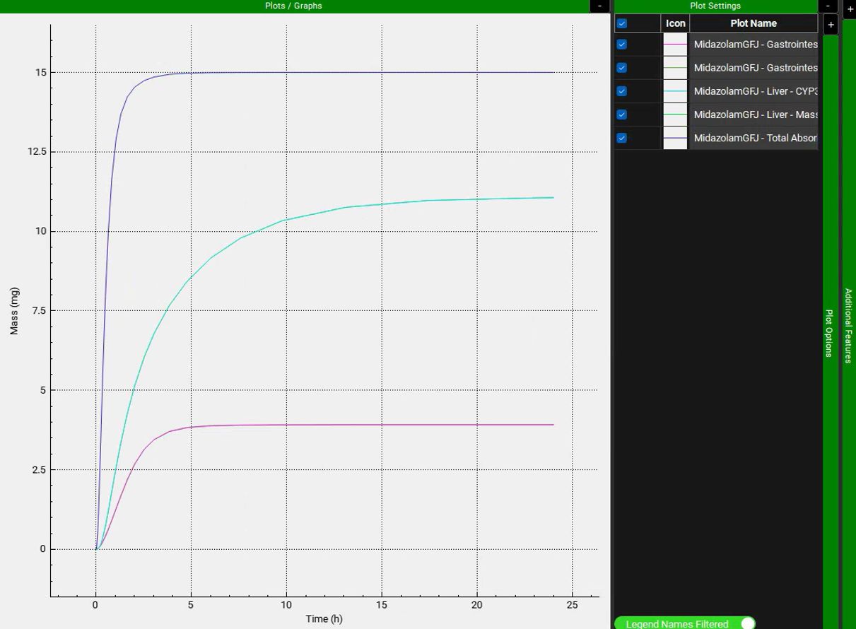
24. Collapse the Additional Features by clicking on the “-” and expand the Plot Settings by clicking on the “+” on top of the bar. The legend will be displayed. Enable the Legend Names Filtered toggle at the bottom. Drag and expand the Plot Settings panel to see the entire legend names. Notice how there are two lines for Enterocytes (labelled as Epithelial) and Liver plotting the Total Mass Metabolized and the Mass Metabolized by CYP3A4. Since all metabolism is coming from CYP3A4, these lines are overlaid.

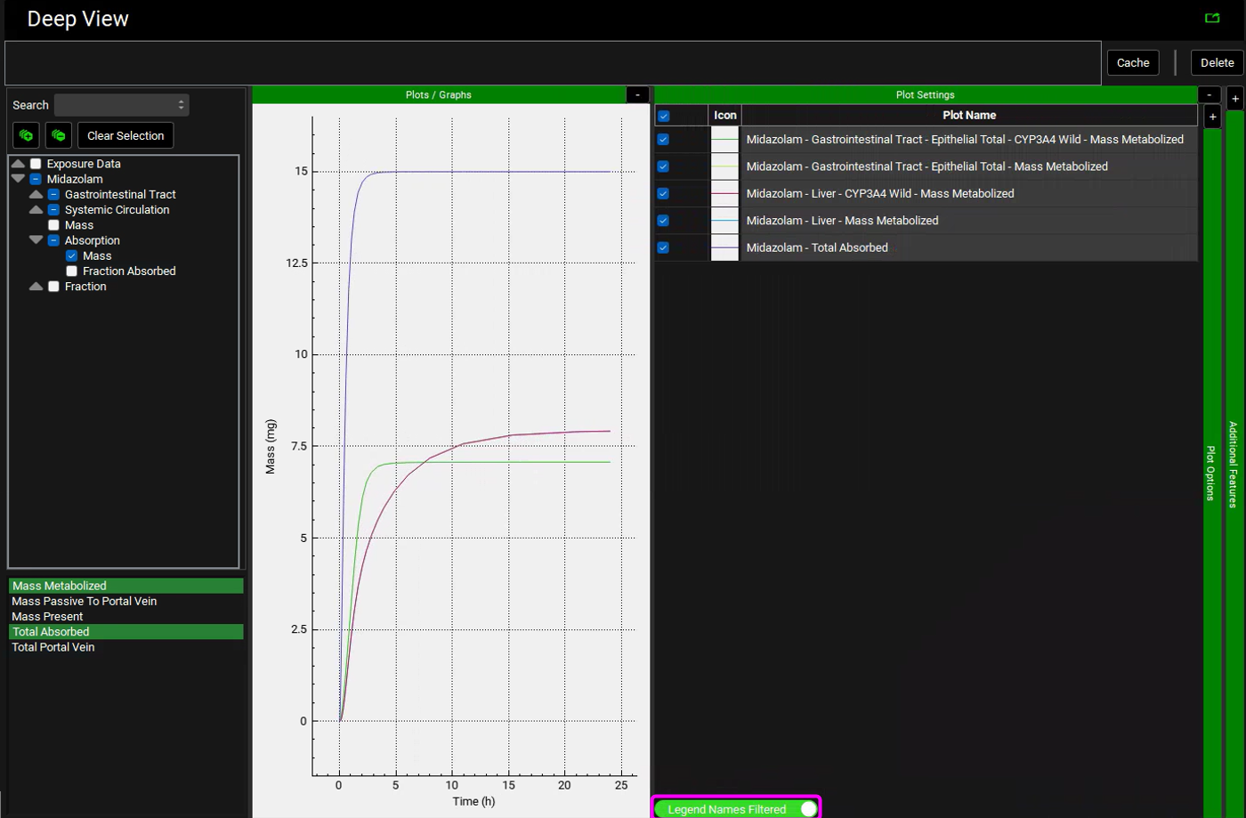
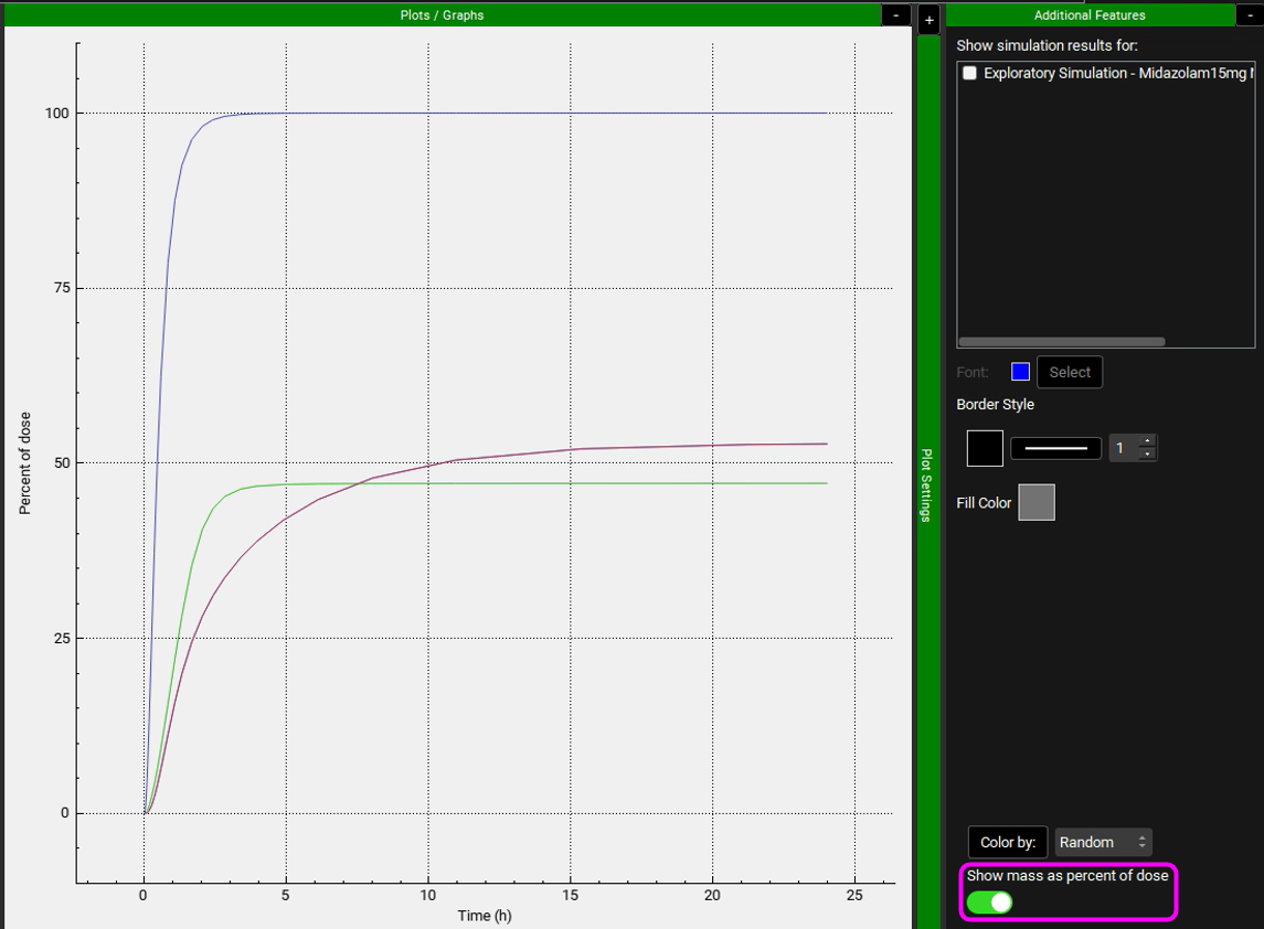
Note that the simulation predicts approximately 47% of the drug was metabolized in the gut, and approximately 53% was metabolized in liver. According to the literature, gut and liver metabolism should be nearly equal for this dose. To display Mass as a Percent of dose, expand the Additional Features panel and turn on the Show mass as percent of dose toggle, found at the bottom, the toggle will turn green when it is on.

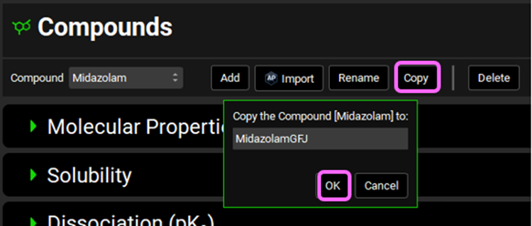
25. Navigate to the Compounds view and Copy the Midazolam compound. Name the new compound MidazolamGFJ and click OK. We will set this compound up to reflect dosing in the presence of Grapefruit Juice.

26. Open the Enzymes Kinetics panel and reduce the Enterocytes V_max from 0.2631 to 0.1 mg/s (62% less) by clicking on the cell and typing 0.1 (keep the mg/s unit) and hit enter. If necessary, use CTRL A to select the whole value in the cell before entering the new value.

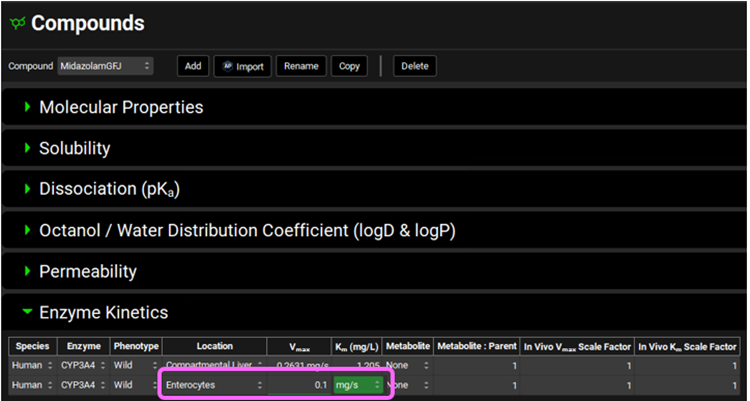
This is in agreement with the observations of Lown et al. ³ where GFJ ingestion reduced gut 3A4 activity by 62% without any change in the m-RNA levels.

*Do not change the liver V_max – GFJ only affects gut 3A4 levels.

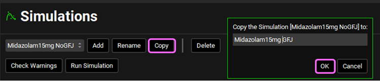
27. Navigate to the Simulations view and Copy the Midazolam15mg NoGFJ simulation. Name the new simulation Midazolam15mg GFJ and click OK.

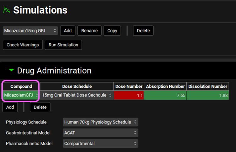
28. Switch the Compound to MidazolamGFJ from the Compound drop-down in the Drug Administration panel.

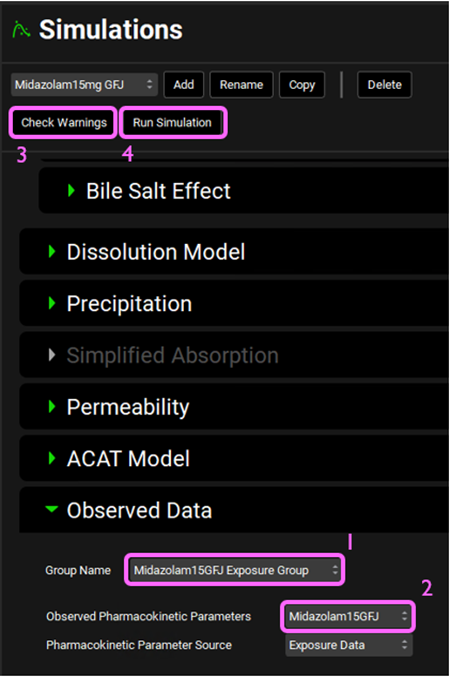
29. Expand the Compound Settings panel and scroll down to the Observed Data sub-panel, expand it, and select Midazolam15GFJ Exposure Group from the Group Name drop-down. Select Midazolam15GFJ from the Observed Pharmacokinetic Parameters drop-down. Then, click on Check Warnings and Run Simulation at the top of the Simulations view.

30. Once the simulation finishes, the program switches automatically to the Analysis view.

31. Examine the C_p-Time curve in the Kew View.

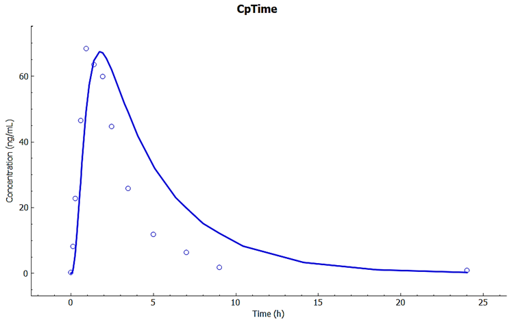
Observe how the predicted C_p-Time is close to the observations using the same absorption and PK model, with only the V_max in gut changed to agree with the literature observation that 3A4 metabolism is reduced by about 62% because of grapefruit juice.

32. Repeat steps 22-24 to compare the gut and liver metabolism amounts. Observe how the gut metabolism is now only about 1/3 of liver metabolism.

Metabolite Tracking

This tutorial describes how to set up a GPX™ Project and Simulations for the pharmacokinetics of a parent compound as well as its metabolite(s). This feature requires the GPX™ Metabolism and Transport (M&T) module. Metabolite tracking can be included in your simulation with either a PBPK model (demonstrated in Example 1 of this tutorial) or a Compartmental PK model (demonstrated in Example 2 of this tutorial). If you have not yet run the tutorials for corresponding modules (Metabolism and Transporter module and the PBPKPlus™ Module Tutorial or PKPlus™ Module Tutorial, respectively), we suggest that you run them first.

Example 1: PBPK Model

This example requires the GPX™ PBPKPlus™ module. If you are not licensing PBPKPlus™, proceed to Example 2 to see how to set up metabolite tracking with a Compartmental PK model.

1. Open GPX™ and, in the Dashboard view, click on the icon next to Select to open an Existing project.

2. Click Browse and navigate to the C:\Users\<user>\AppData\Local\Simulations Plus, Inc\GastroPlus\10.2\Tutorials\Metabolite Tracking and select the project file Metabolite Tracking.gpproject by clicking on it and clicking Open.

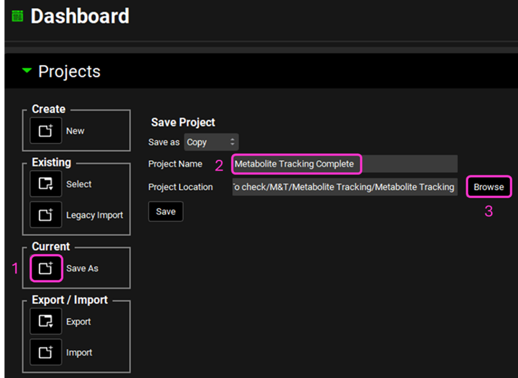
3. Save a copy of the project by clicking on the icon next to Save As, entering “Metabolite Tracking Complete” as the Project Name and click Browse to navigate to/add a folder to Save the project in. You will see an information message in the Messages Center indicating that the project has been successfully copied. This message will disappear once you click 'Yes' on the pop-up window. Note that the name of the project visible in the top right corner of the interface is the one that has just been created.

4. Navigate to the Observed Data view and note that there are four data entries in the Summary of Data Profiles sub-panel table. All four Data Types are Exposure Data. Each Group Name (Metoprolol and Metabolite) has two Series, representing the plasma concentration profile (Measurement Type: Concentration) and Urine data (Measurement Type : Mass).

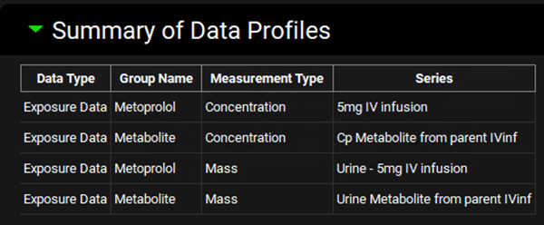
5. Select Metoprolol from the Group Name drop-down under the Profiles panel and scroll down to the mapping table located below the Plot. See how both Series have been mapped to their specific compartment (Venous Return and Urine). Do the same for the Metabolite Group Name and observe the data mapping.

This project contains the C_p-Time profile for metoprolol and metabolites after intravenous administration (10 min infusion) of 5 mg of metoprolol tartrate. This would correspond to administration of 3.9 mg of metoprolol alone.

The clinical data for this intravenous study comes from Regårdh et al. ⁴ The data assigned to α-hydroxymetoprolol is the sum of all metabolites. Cumulative urinary excretion for unchanged and total metabolites from Regardh are included in the Observed Data view.

6. Navigate to the Compounds view where you can see the physicochemical and biopharmaceutical properties of the compounds that were imported/created. This project contains three compounds: Metoprolol AP 11.0 (ADMET Predictor^® import), Metoprolol In vitro (mix of in vitro properties and in silico predictions), and a-OH-Metoprolol (ADMET Predictor^® import).

Please refer to the Compound and ADMET Predictor® sections in the Lab Book for more information.

7. In the Compounds view select Metoprolol In vitro from the Compound drop-down. Expand the panels by double-clicking on the panel header or clicking on the green arrow. Review those properties and observe that metoprolol is a strong base with pKa ~ 9.7, moderate permeability, and high solubility (8.51 mg/mL) at pH 11.04 at 25^οC.

8. Select a-OH-Metoprolol (metabolite) and review its properties in the Compounds view.

9. Navigate to the Dosing view and review the Formulations and Dosing Schedules panels. In this project there is one Formulation (IV infusion) and one Dosing Schedule (3.9mg IV infusion).

10. Navigate to Physiologies view and note that there is a Human 78kg 30y physiology created.

11. Navigate to Pharmacokinetics view. Make sure that Metoprolol In vitro is chosen from the Compound drop-down. Notice how both Compartmental and PBPKPlus™ models are available.

12. Expand the PBPKPlus™ panel. Metoprolol is cleared mainly by metabolism, but a small amount of parent drug is also secreted in urine. For drugs without contribution of active tubular secretion or a significant reabsorption, the renal clearance can be estimated from glomerular filtration rate (GFR) and drug binding in plasma. Select the Kidney tissue in the PBPK diagram and scroll down to the Urine sub-panel on the right-hand side of the diagram (it may be easier if the Physiology panel is collapsed). If necessary, expand the Urine sub-panel and note how the Kidney Filtration Method is set to F_up * GFR. The program will automatically calculate the filtration clearance (F_up * GFR (mL/s)).

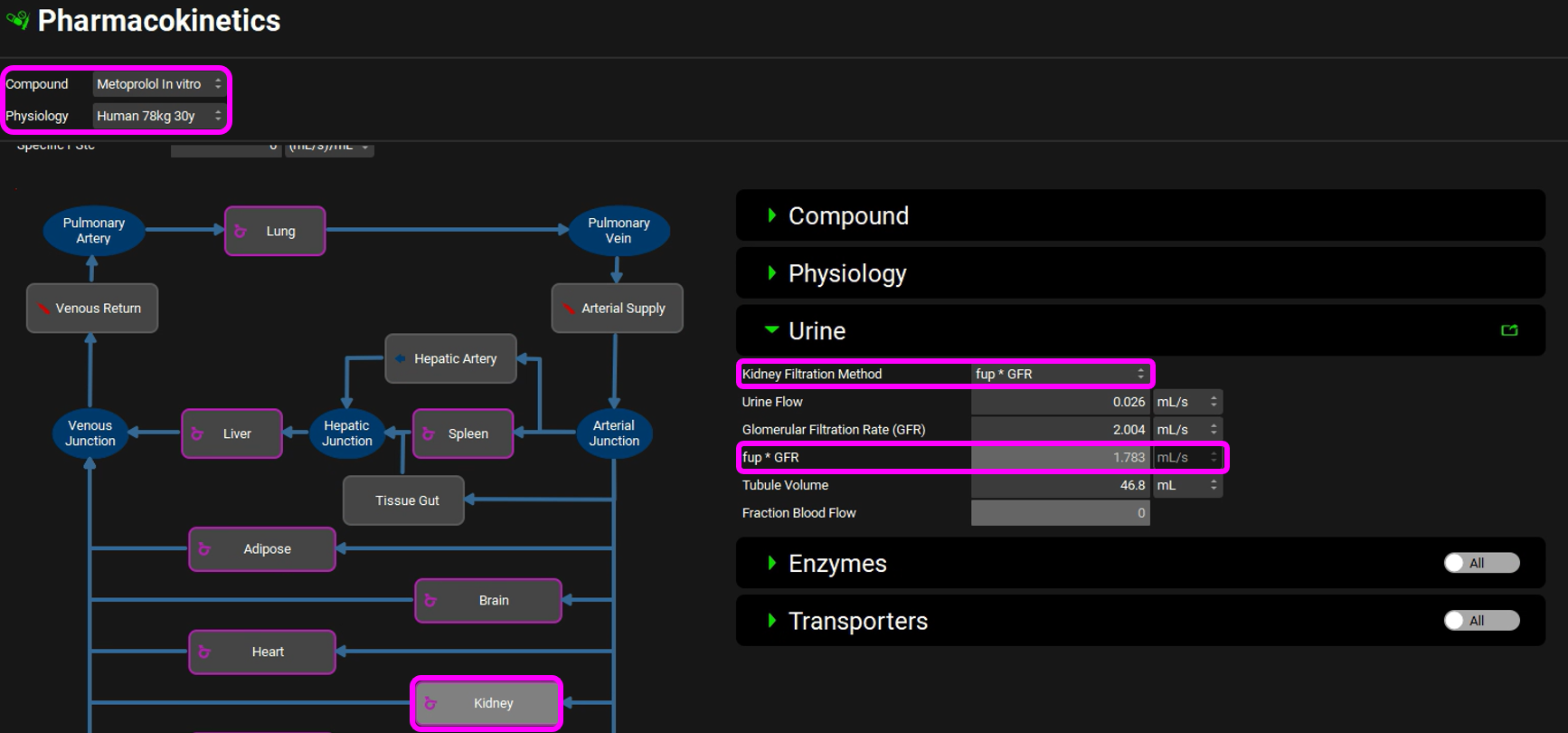
13. Scroll down to the PBPK table to see the renal filtration clearance displayed in the CL (L/h) column of the PBPK table.

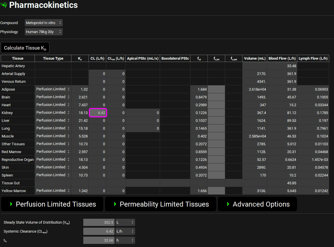
The units can be changed in the CL (L/h) column by clicking on the units in the column header and selecting mL/s to confirm the table matches the renal filtration clearance.

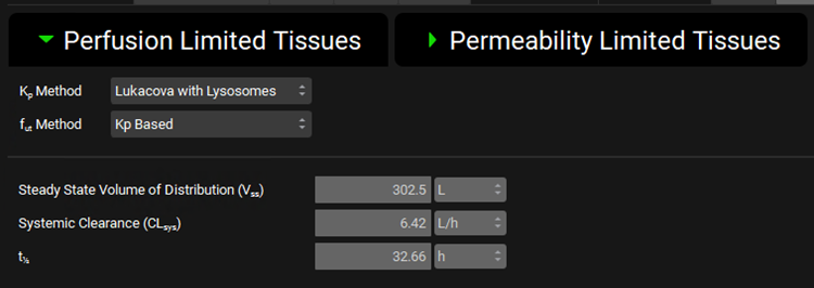
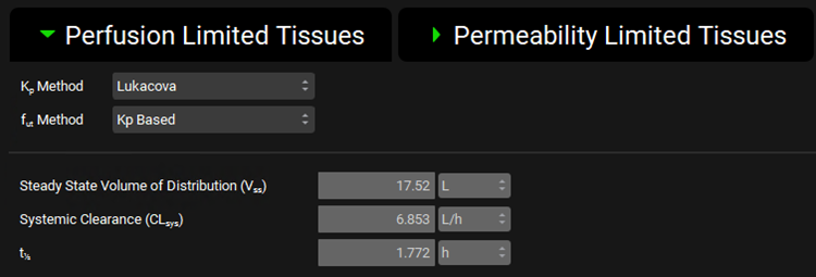
14. Expand the Perfusion Limited Tissues sub-panel under the PBPK panel and note that the Lukacova with Lysosomes Kp calculation method has been chosen for Vss calculation.

15. Scroll up to the top of the Pharmacokinetics view and switch the Compound to a-OH-Metoprolol. Note the Blood Plasma Concentration Ratio and Experimental F_up for this compound.

16. Expand the PBPKPlus™ panel if not already expanded. Select the Kidney tissue in the PBPK diagram and, if necessary, expand the Compound panel (on the right-hand side of the diagram) note that the kidney Apical PStc has been set to 0.005 mL/s to account for some reabsorption to capture the observed urinary excretion data.

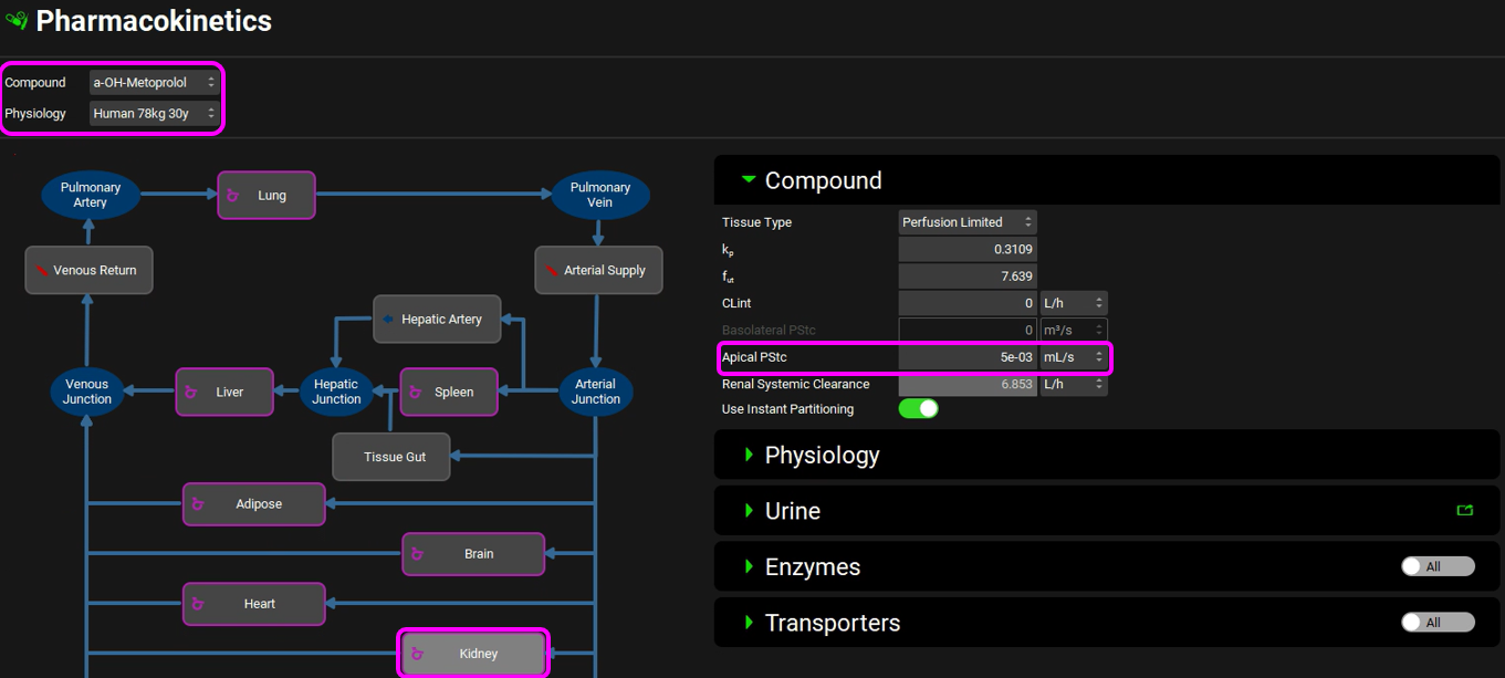
17. Scroll down to the Urine sub-panel and note that the Kidney Filtration Method is also set to F_up * GFR. The program will automatically calculate the filtration clearance (F_up * GFR (mL/s)) (Considering F_up = 95%)

18. Scroll down to the PBPK table to see the renal filtration clearance displayed in the CL (L/h) column of the PBPK table.

19. Expand the Perfusion Limited Tissues sub-panel under the PBPK panel and note that the Lukacova Kp calculation method has been chosen because most of these metabolites will be glucuronides.

V_ss was calculated using F_up = 20% and then changed to 95% for the simulation.

20. Switch the compound back to Metoprolol In vitro. We will now add enzyme entries to the Enzyme Kinetics table.

Since we will be creating both PBPK and compartmental simulations, we need to put 2D6 into both Tissue (PBPK) and Liver (Compartmental). The K_m value comes from an in vitro metabolic study by Madani et al. and the V_max value for this study was fitted to an average value for a mixed population of polymorph expression.

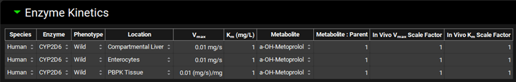
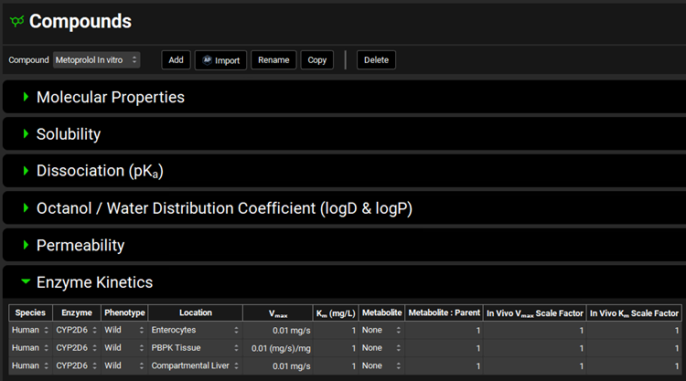
21. Navigate to the Compounds view, expand the Enzyme Kinetics panel, and click Add (located at the bottom of the panel). An entry will be created in the table. Metoprolol is a substrate of CYP2D6, so choose CYP2D6 from the Enzyme drop-down and select Enterocytes from the Location drop-down. Click Add again and choose CYP2D6 from the Enzyme drop-down. Select PBPK Tissue from the Location drop-down. Click Add again, choose CYP2D6 from the Enzyme drop-down and leave Compartmental Liver selected from the Location drop-down.

22. Select a-OH-Metoprolol from the Metabolite drop-down for each row.

23. Save the project, using the Save button in the top right corner of the interface and click on OK on the Save completed message.

24. Navigate to the Metabolism & Transport module via the Modules pane on the right-hand side of the interface.

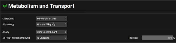
25. Select Metoprolol In vitro from the Compound drop-down, select User Recombinant from the Assay drop-down and Is Unbound from the In Vitro Fraction Unbound drop-down.

26. Expand the Scaling Factors panel and select PBPK from the Tissue Weight Source drop-down.

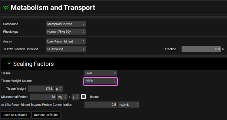
We will assume a 1738 g liver weight for the PBPK liver. This value can be edited in the Scaling Factors panel.

If the In Vitro Recombinant Enzyme Protein Concentration box appears empty, you can either click on the Restore Defaults button (as the default value is used in this tutorial) or you can either type directly the value in the box.

27. Expand the Metabolism panel and leave all the defaults in the Enzyme-Specific table.

28. Expand the Michaelis-Menten Kinetics sub-panel to enter the in vitro rCYP2D6 enzyme parameters.

Leave In Vitro selected from the V_max Type drop-down. Select pmol/min/pmol before entering the in vitro V_max (V_max = 42 pmol/min/pmol CYP). Select µmol/L as the unit for In vitro K_m and then enter the K_m value of K_m = 26 µM.

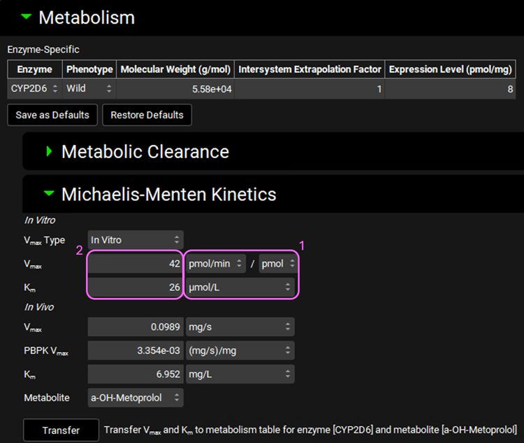
The converted in vivo enterocyte V_max should be 0.0989 mg/s, the PBPK V_max should be 3.354E-3 mg/s/mg Enz, and the in vivo K_m should be 6.952 mg/L.

In the Scaling Factors panel of the M&T Module, be sure that the “Tissue Weight Source” is PBPK not Compartmental.

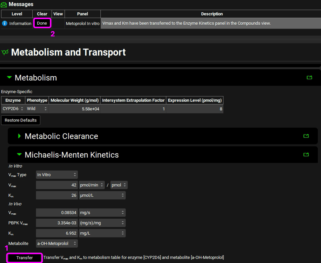
29. Click on the Transfer button to Transfer V_max and K_m to the Enzymes Kinetics in the Compounds panel. A message will appear in the Messages center informing that the V_max and K_m have been transferred. Click Done to clear the message.

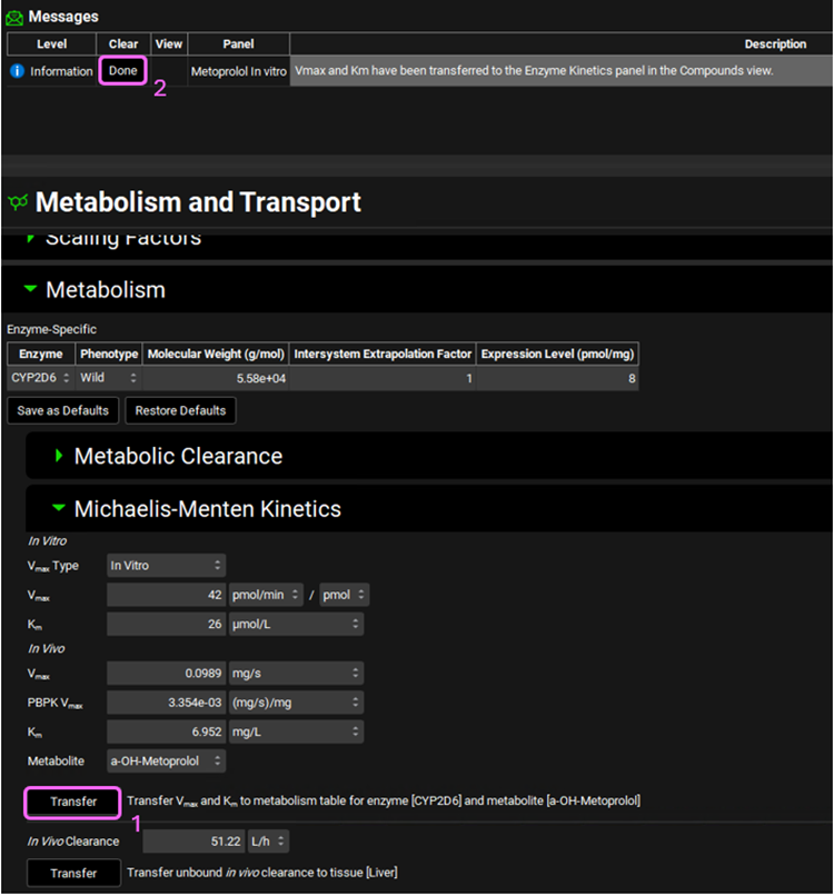
You can use the pop-out functionality (by clicking the green icon at the right side of the panel) to see the Enzyme Kinetics panel (from the Compounds view) and the M&T module at the same time. Closing (X) the pop-up window will bring the Enzyme Kinetics panel back to Compounds view.

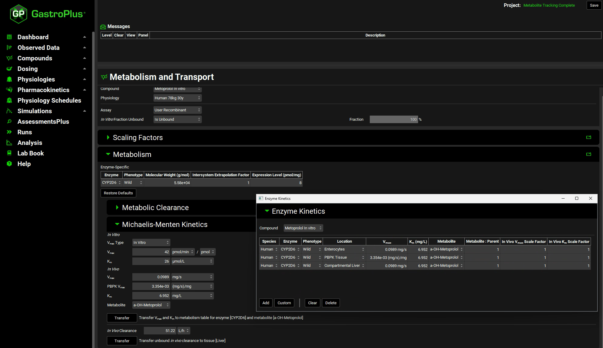
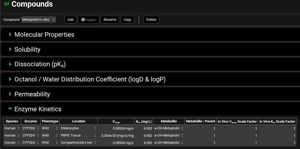
30. Navigate to the Compounds view to see the in vivo K_m and V_max values transferred to the Enzyme Kinetics table.

31. Navigate to the Physiologies view and open the Gastrointestinal panel and scroll down to the Enzyme and Transporter Distribution table to view the gut distribution and confirm that it matches the following table:

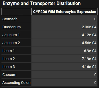
GastroPlus® will scale the absolute values of the gut distribution depending on the body weight up to 78 kg. After that the values are assumed to be constant at the adult level. The turnover rates in min^-1 for the enzyme in each compartment can be viewed, edited, and saved in Physiologies/ Gastrointestinal/Enzymes sub-panel to the right of the GI diagram. These are used in drug-drug interaction prediction for time-dependent inhibitors.

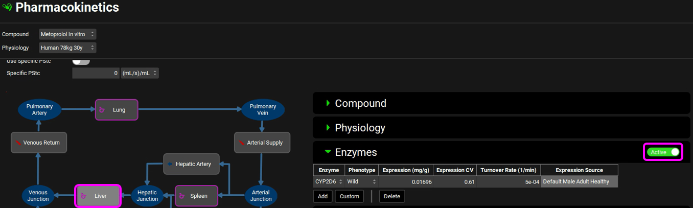
The Liver enzyme Expression, CV and Turnover Rate can be seen in the Pharmacokinetics view. Select the Liver tissue in the PBPK diagram and scroll to the Enzymes sub-panel to the right of the diagram. In the Enzymes sub-panel you can click on the Active toggle so that only the enzymes included in the model will be shown in the list.

31. Save the project and click OK.

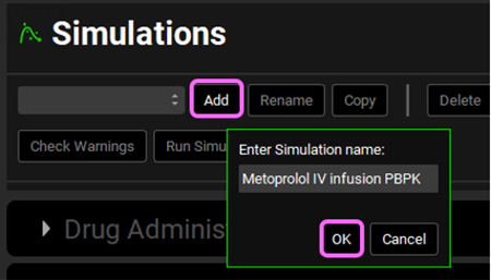
32. Now we are ready to start a Simulation. Proceeding down the navigation pane, click on the Simulations view. Click on Add and type Metoprolol IV infusion PBPK in the Enter Simulation name dialog box then click OK.

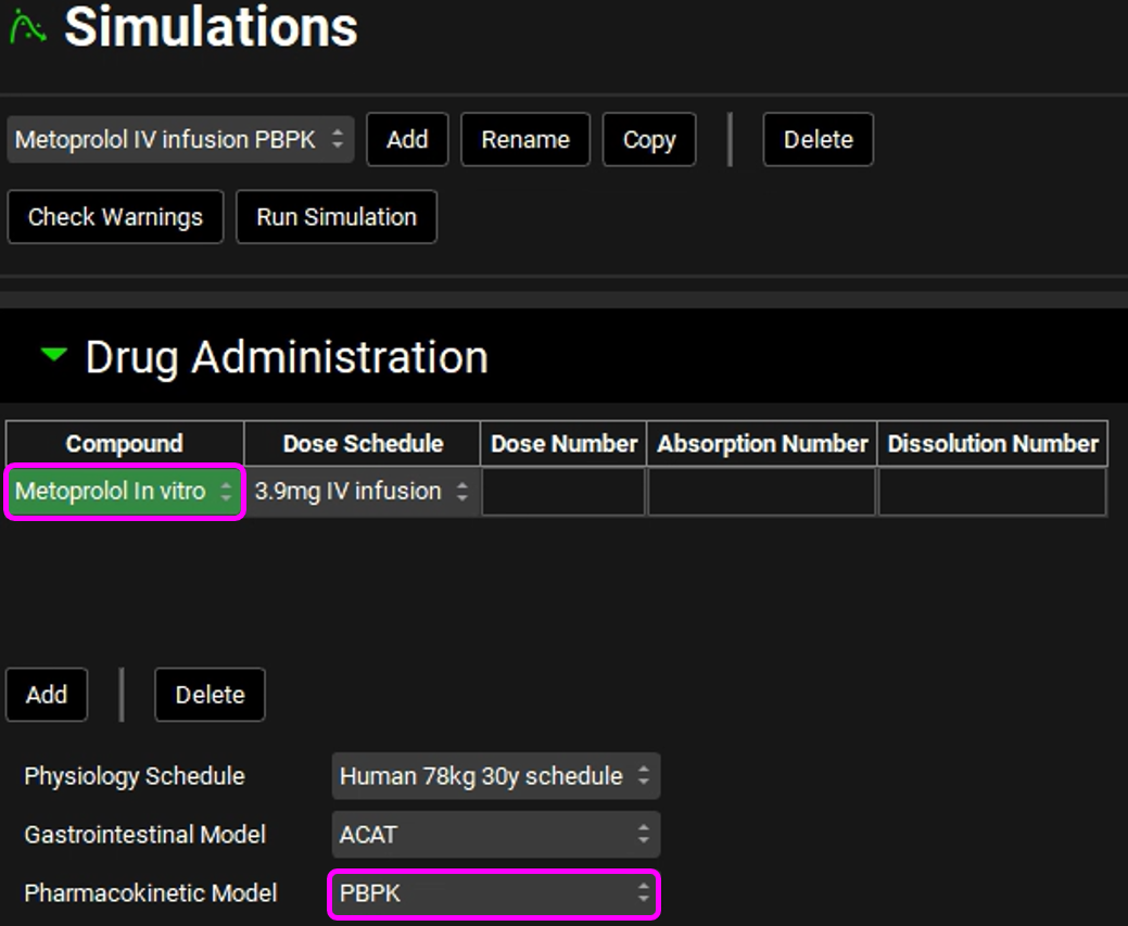
33. Expand the Drug Administration panel and select Metoprolol In vitro from the Compound drop-down. As there is only one Dose Schedule and Physiology Schedule in the project, 3.9mg IV Infusion and Human 78kg 30y schedule should automatically be selected. Set the Pharmacokinetic Model to PBPK. Click Done to clear the warning message about Liver FPE.

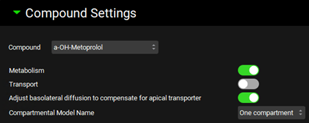
34. Expand the Compound Settings panel and make sure that Metoprolol In vitro is selected from the Compound drop-down. Ensure the Metabolism toggle is on.

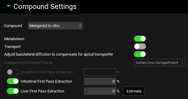
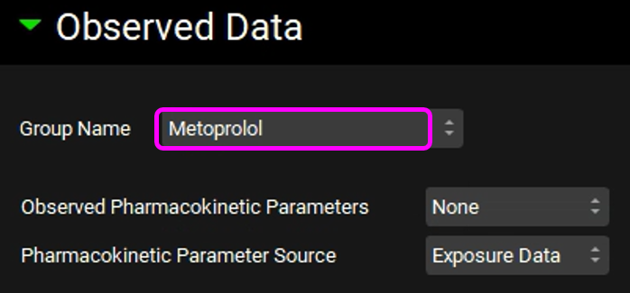
35. Scroll down to the Observed Data sub-panel and select Metoprolol from the Group Name drop-down.

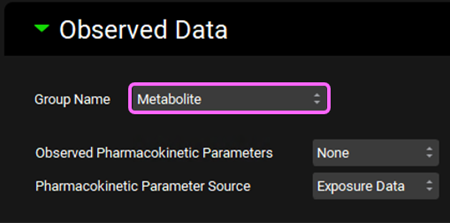
36. Navigate back to the top of the Compound Settings panel and switch the Compound to a-OH-Metoprolol.

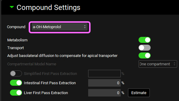
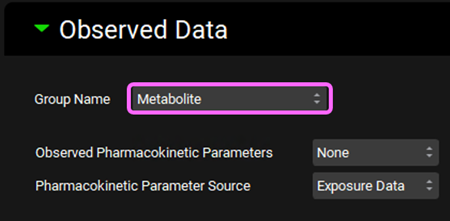
37. Scroll down to the Observed Data sub-panel and select Metabolite from the Group Name drop-down.

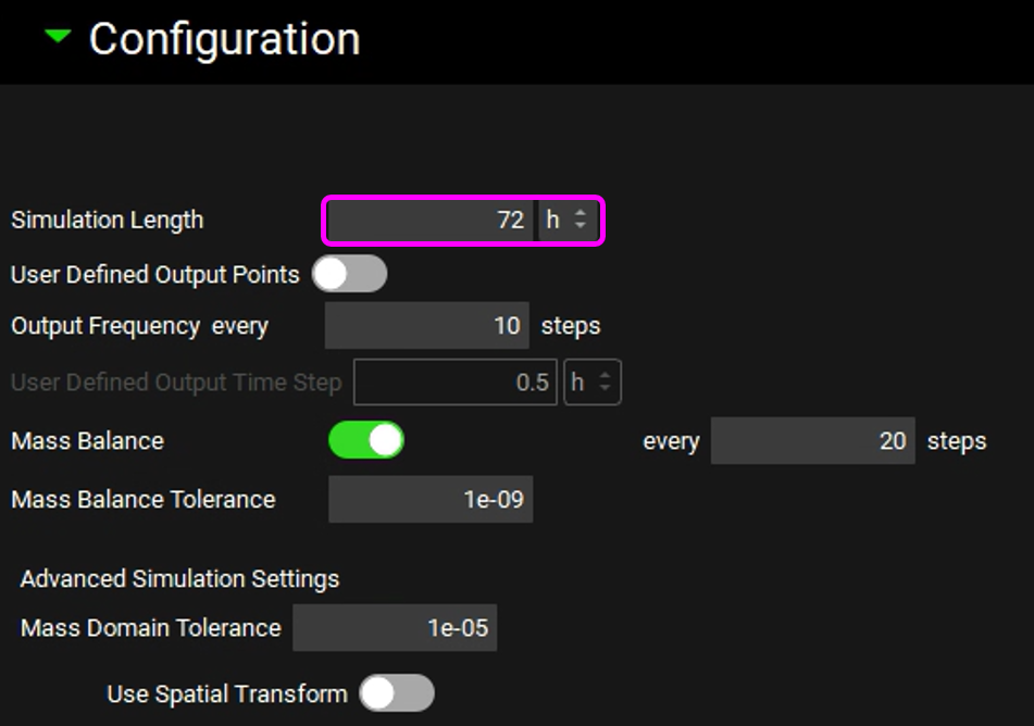
38. Open the Configuration panel and set the Simulation Length to 72h.

39. Save the project and click OK.

40. At the top of the Simulations View, click Check Warnings then Run Simulation.

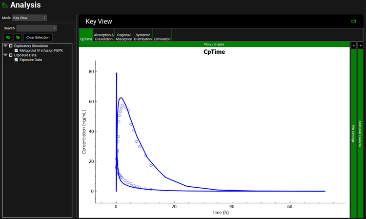
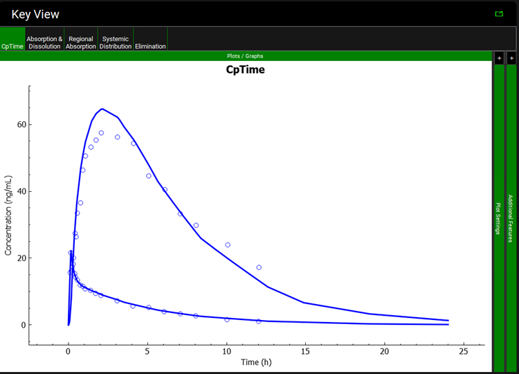
41. Once the simulation finishes, the program switches automatically to the Analysis view. The C_p-Time plot will be displayed in the Key View mode.

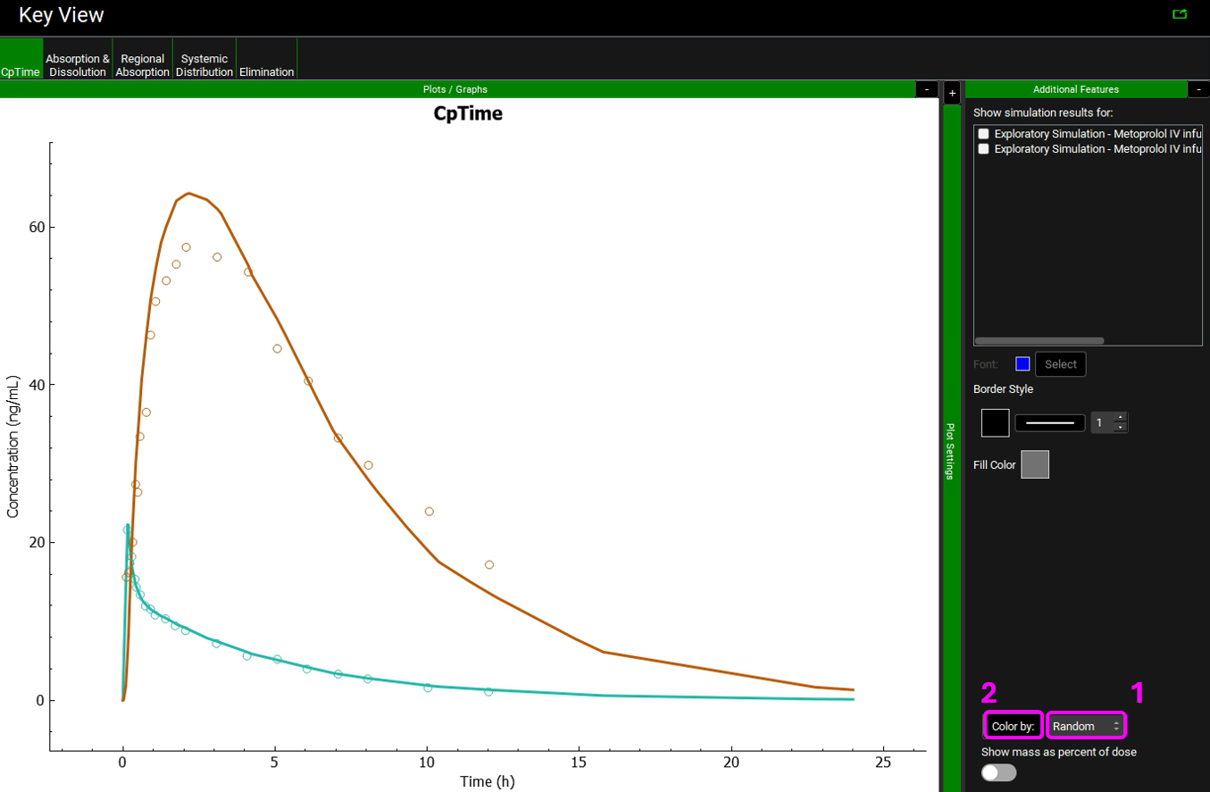
42. Expand the Additional Features panel by clicking on “+” at the top of the bar on the right-hand side of the graph. Select Compound from the drop-down (default selection is Tissue) and then click on the Color by button.

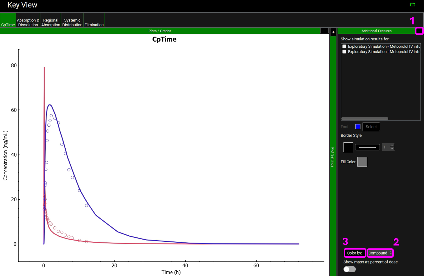
Notice that the simulation is a very good estimate of the actual human C_p-Time.

43. Move to the Elimination plot in the Kew View ribbon. The Urine data is shown in yellow.

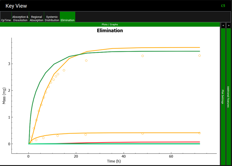
You can recolor the urine data to differentiate between Parent and Metabolite.

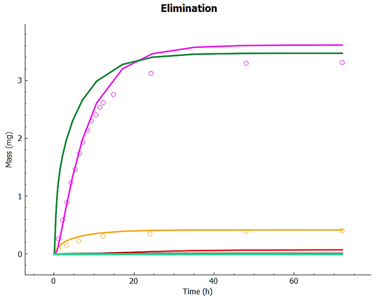
Examine the match between simulated and observed data for each dataset. Notice the good overall agreement. Since the expression of 2D6 is highly variable, it can be expected that the 2D6 expression may need to be adjusted for different groups of subjects.

44. Compare the Observed and Simulated C_p vs. time profiles in Key View. Study the other plots from the Key View ribbon. For a summary of the C_max, T_max, and AUC values you may select the Summary View from the Mode drop-down.

45. Now we will go into the Deep View to see the C_p-Time plot that includes the Urinary excretion for unchanged metoprolol and its metabolite (α-hydroxymetoprolol).

46. Select Deep View from the Mode drop-down.

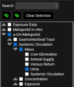
a. Expand a-OH-Metoprolol in the series list tree by clicking on the grey arrow. Select the following series from the list by clicking in the checkbox next to the series name:

a-OH-Metoprolol ->Systemic Circulation->Mass->Urine. (You can also use the search bar by typing Urine)

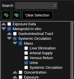
b. Collapse the a-OH-Metoprolol series and expand Metoprolol In vitro in the series list tree by clicking on the grey arrow. Select the following series from the list by clicking in the checkbox next to the series name:

Metoprolol In vitro ->Systemic Circulation->Mass->Urine (You can also use the search bar by typing Urine)

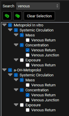
c. Type “Venous” in the Search box and press Enter. Select the Venous Return under Concentration branch for both a-OH-Metoprolol and Metoprolol In vitro.

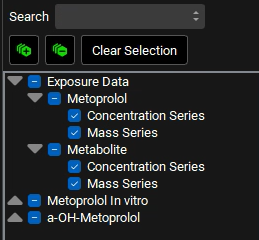
d. Delete the text in the Search box and press Enter. Collapse all sections by clicking on the  icon. Expand Exposure Data in the series list tree by clicking on the grey arrow. Select both Concentration Series and Mass Series for Metoprolol and Metabolite by clicking in the checkbox next to the series name.

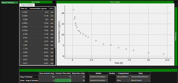
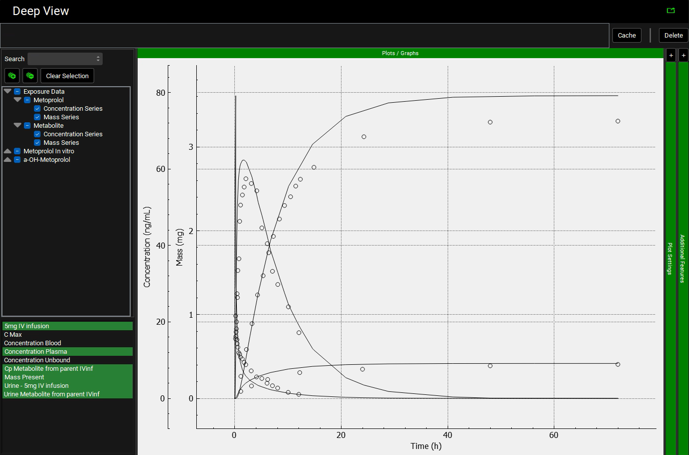
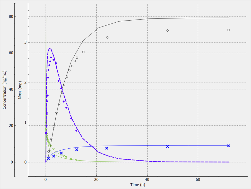
In the variables list at the bottom, select 5mg IV infusion and then hold down CTRL and click on Concentration Plasma, C_p Metabolite from parent IVinf, Mass Present and both Urine data.

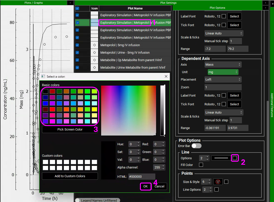
47. Expand the Plot Settings by clicking on the “+” on top of the bar. The legend will be displayed. Click on the simulated line with the higher amount in urine and hover over the highlighted Plot Name in the legend. You will notice that this curve is related to the metabolite.

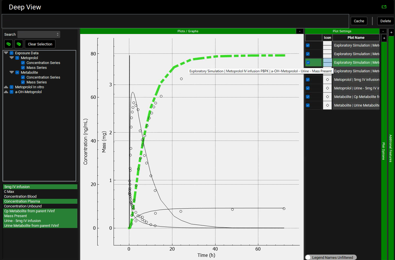
48. Similarly, click on the observed data (circles) with the higher amount in urine and hover over the highlighted Plot Name in the legend. You will notice that this curve is also related to the metabolite.

49. We will leave the metabolite simulated line and observed data (circle) in black for both plasma concentration and Urine data and will assign different colors to the parent compound (Metoprolol). Hover over the Plot Name to see the entire name and select the Metoprolol In vitro simulation (line). Expand the Plot Options by clicking on the “+” on top of the bar. Scroll down to the Line frame and click on the Color square next to Options. Select a color different than black and click OK.

50. Select the observed data (circles) for Metoprolol. In the Plot Options panel, scroll down to the Points frame and click on the Color square next to Line options. Select the matching color and click OK.

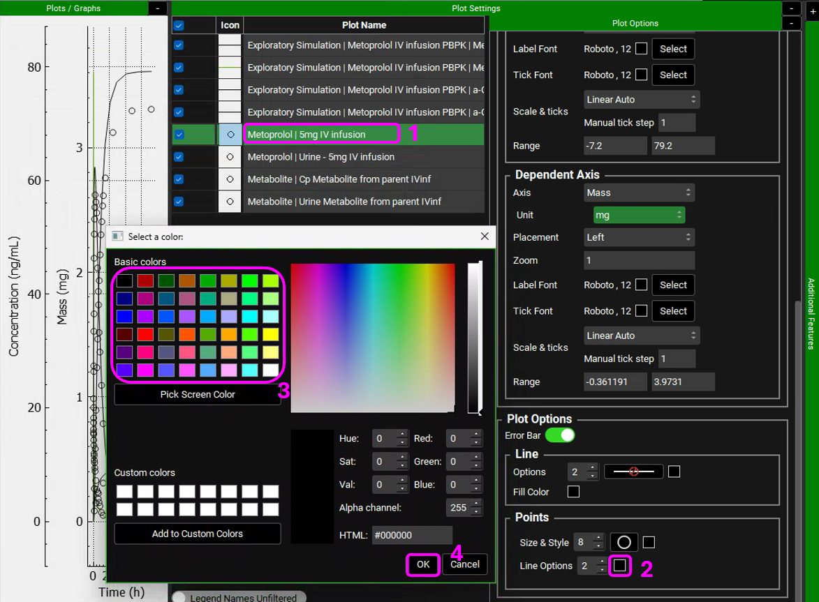
You can also edit the Shape of the observed data Points to differentiate between Urine and Plasma data.

Metoprolol is cleared mainly by metabolism, but a small amount of parent drug is also secreted in urine. However, the urinary excretion of the metabolites is quite high as shown above. For drugs without contribution of active tubular secretion or a significant reabsorption, the renal clearance can be estimated from glomerular filtration rate (GFR) and drug binding in plasma.

Example 2: Compartmental PK Model

We will run the same exercise as Example 1 but we will use a compartmental PK model instead of a full PBPK model.

1. Navigate to the Pharmacokinetics view. Make sure that Metoprolol In vitro is chosen from the Compound drop-down. Notice how both Compartmental and PBPKPlus™ models are available.

2. Expand the Compartmental panel to see the one compartmental model linked to this compound. These parameters were obtained when the compound structure was imported (ADMET Predictor^® module predicts the clearance and V_c for this model).

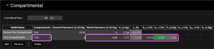
3. We will now manually add the PK parameters that were obtained by fitting the Metoprolol IV infusion data in PKPlus™. Click on Add button located below the table and type Two Compartments in the Enter model name dialog box then click OK.

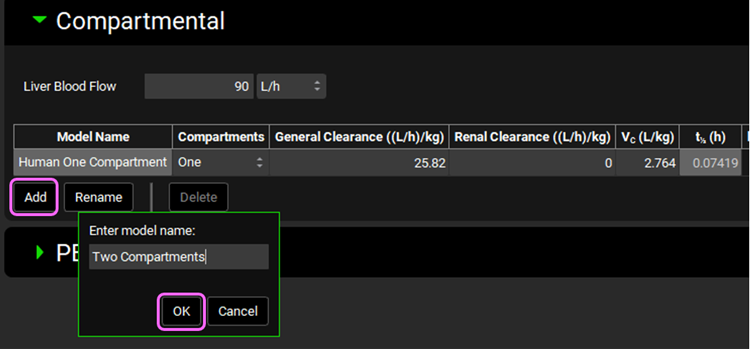
4. Select Two from the Compartments drop-down. Metoprolol is mainly cleared by CYP2D6 metabolism, with a small contribution of renal secretion. We will use these clearance mechanisms to specify metoprolol elimination instead of CL fitted to the in vivo PK profile. Leave the General Clearance as zero and set the Renal Clearance to 0.35 ((L/h)/kg). Set the V_c (L/kg) = 1.771; K12 (1/h) = 2.714; and K21 (1/h) = 2.929.

If the units need to be adjusted, click on the unit in the appropriate column header and select the correct ones, per kg can be activated by checking in the white square.

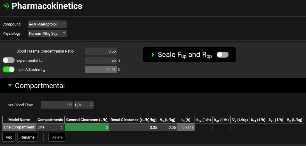
5. Switch the Compound to a-OH-Metoprolol and see the one compartmental model linked to this compound. Leave One compartment selected and set the General Clearance (L/h) =0; Renal Clearance = 0.05 ((L/h)/kg); and V_c (L/kg) = 0.06.

6. Save the project and click OK.

7. If you have already run Example 1 of this tutorial, skip to step 10. If not, proceed to step 8.

8. Navigate to the Compounds view, expand the Enzyme Kinetics panel, and click Add (located at the bottom of the panel). An entry will be created in the table. Metoprolol is a substrate of CYP2D6, so choose CYP2D6 from the Enzyme drop-down and select Enterocytes from the Location drop-down. Click Add again and choose CYP2D6 from the Enzyme drop-down. If you are licensing PBPKPlus™ select PBPK Tissue from the Location drop-down. Click Add again, choose CYP2D6 from the Enzyme drop-down and leave Compartmental Liver selected from the Location drop-down.

If you are not licensing PBPKPlus™ your table will have only two entries (Enterocytes and Compartmental Liver).

9. Select a-OH-Metoprolol from the Metabolite drop-down for all rows.

10. Navigate to the Metabolism & Transport module via the Modules navigation pane on the right-hand side of the interface.

11. Select Metoprolol In vitro from the Compound drop-down, select User Recombinant from the Assay drop-down and Is Unbound from the In Vitro Fraction Unbound drop-down.

12. Expand the Scaling Factors panel and select Compartmental from the Tissue Weight Source drop-down.

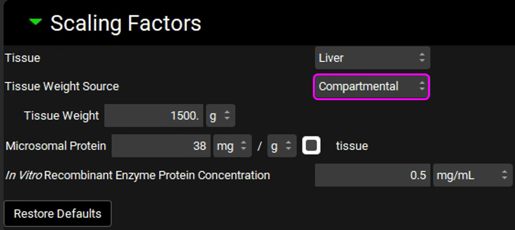
Since we are using a Compartmental PK model, we will assume a 1500 g liver weight for the compartmental simulations.

13. Expand the Metabolism panel and leave all the defaults in the Enzyme-Specific table.

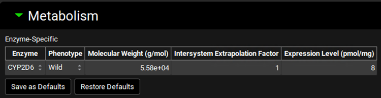
14. Expand the Michaelis-Menten Kinetics sub-panel to enter the in vitro rCYP2D6 enzyme parameters.

Leave In Vitro selected from the V_max Type drop-down. Select pmol/min/pmol before entering the in vitro V_max (V_max = 42 pmol/min/pmol CYP). Select µmol/L as the unit for In vitro K_m and then enter the K_m value of K_m = 26 µM.

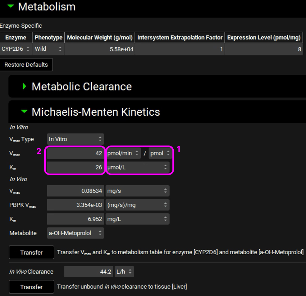
The converted in vivo V_max should be 0.08534 mg/s, and the PBPK V_max should be 3.354E-3 mg/s/mg Enz, and the in vivo K_m should be 6.952 mg/L.

15. Click on the Transfer button to Transfer V_max and K_m to the Enzymes Kinetics in the Compounds panel. A message will appear in the Messages center informing that the V_max and K_m have been transferred. Click Done to clear the message.

16. Navigate to the Compounds view to see the in vivo K_m and V_max values transferred to the Enzyme Kinetics table. Ensure that Metabolite is selected as a-OH-Metoprolol for each row.

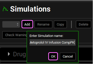
17. Now we are ready to start a Simulation. Proceeding down the Navigation Pane, click on the Simulations view. Click on Add and type Metoprolol IV infusion CompPK in the Enter Simulation name dialog box then click OK.

18. Expand the Drug Administration panel and select Metoprolol In vitro from the Compounds drop-down. As there is only one Dose Schedule and Physiology Schedule in the project, 3.9mg IV Infusion and Human 78kg 30y schedule should automatically be selected. Set the Pharmacokinetic Model to Compartmental.

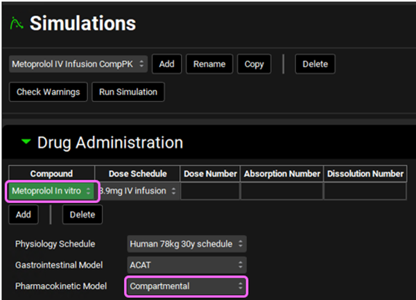
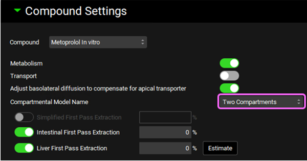
19. Expand the Compound Settings panel and make sure that Metoprolol In vitro is selected from the Compound drop-down. Ensure the Metabolism toggle is on and select Two Compartments from the Compartmental Model Name drop-down. Click Done to clear the warning message about Liver FPE.

20. Scroll down to the Observed Data sub-panel and select Metoprolol from the Group Name drop-down.

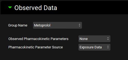
21. Navigate back to the top of the Compound Settings panel and switch the Compound to a-OH-Metoprolol.

22. Scroll down to the Observed Data sub-panel and select Metabolite from the Group Name drop-down.

23. Save the project.

24. At the top of the Simulations View, click Check Warnings then Run Simulation.

25. Once the simulation finishes, the program switches automatically to the Analysis view in the Key View mode. Select the C_p-Time plot from the Key View ribbon, if it isn’t already displayed.

26. Expand the Additional Features panel by clicking on “+” at the top of the bar on the right-hand side of the graph. Select Random from the drop-down (default selection is Tissue) and then click on the Color by button.

Notice that the simulation is a very good estimate of the actual human C_p-Time.

The colors in your graph might be different.

Transporter-based IVIVE - Metabolism and Transporter module 

This tutorial describes the transporter-based IVIVE (in vitro-in vivo extrapolation) method unique to GastroPlus®, which accounts for scaling of both carrier-mediated and passive transport processes. This feature requires the Metabolism and Transporter module.

The strategy highlighted in this tutorial is to first use rat in vivo and in vitro data in order to refine the PBPK model and then apply it to human.

This tutorial requires PBPKPlus™ license.

PART 1 – Preclinical PBPK model

1. Open GPX™ and, in the Dashboard view, click on the icon next to Select to open an Existing project.

2. Click browse and navigate to the to C:\Users\<user>\AppData\Local\Simulations Plus, Inc\GastroPlus\10.2\Tutorials\GPX Valsartan and select the project file GPX Valsartan.gpproject by clicking on it and clicking Open.

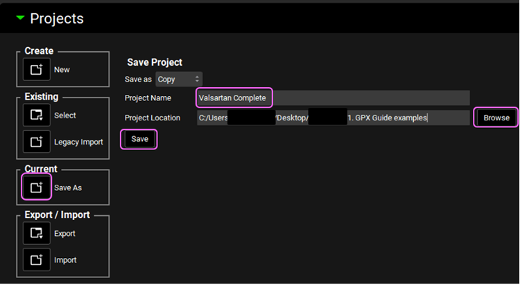
3. Save a copy of the project by clicking on the icon next to Save As, entering “Valsartan complete” as the Project Name and click Browse to navigate to/add a folder to Save the project in. You will see an information message in the Messages Center indicating that the project has been successfully copied. This message will disappear once you click 'Yes' on the pop-up window.
   Note that the name of the project visible in the top right corner of the interface is the one that has just been created.

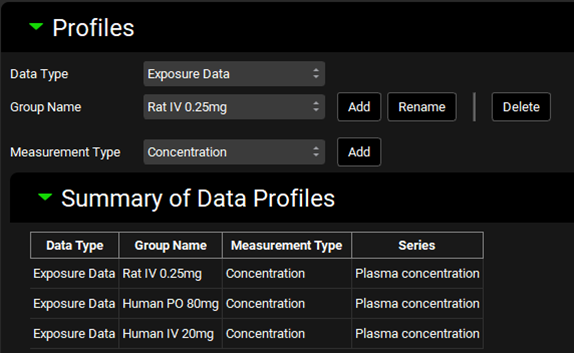
4. Navigate to the Observed Data view in the navigation pane and then review the Exposure Data. This project contains Exposure Data of plasma concentration versus time profiles for rat (intravenous) and human (intravenous and oral).

5. Navigate to the Compounds view in the navigation pane and click on Valsartan_AP11.0 to review the in silico predictions in each panel for Valsartan.

6. Select Valsartan In Vitro from the Compound drop-down. This asset has experimental information for logP, acid pKas and adjusted permeability. The F_up and R_bp in the Pharmacokinetic view has also been obtained from literature by Poirier ⁵ .

7. All other properties are predicted.

8. Navigate to the Dosing view in the navigation pane and review the dosing schedules 0.25mg IV bolus and 20mg IV bolus.

9. Navigate to the Physiologies view to see the physiologies for both rat and human. Set the physiology to Rat 0.25kg and make sure that Valsartan In Vitro is selected.

10. Expand the Population Estimate for Age-Related Physiology (PEAR) by double clicking the panel header or clicking on the green arrow. Observe the existing PEAR physiology for Rat.

11. Switch the physiology to Human 85.53kg 30yo from the Physiology drop-down and observe the existing human PEAR physiology.

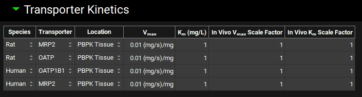
12. Navigate back to the Compounds view and with Valsartan In Vitro selected, expand the Transporter Kinetics panel. Valsartan is reported to be taken up into hepatocytes mainly via OATP transporters and actively excreted by MRP2 ⁶ .

Because GastroPlus® currently does not have built-in expression levels of OATP in any of the rat tissues, the OATP transporter does not appear in the transporter drop-down by default. However, you may add any transporter to your model by simply creating a custom transporter.

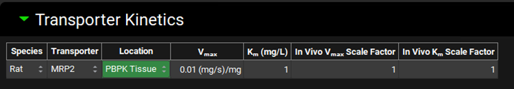
13. If not available, click on Add (located at the bottom of the Transporter Kinetics table) to create a table entry, switch the Species to Rat and select MRP2 from the Transporter drop-down. Select PBPK Tissue from the Location drop-down.

14. Next, if not available we will create a custom transporter. Click on Custom to create an entry for the OATP transporter. The Enter custom transporter name: dialog box will appear. Select Rat from the drop-down and type OATP as the name of the transporter. Then click OK.

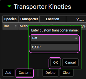
15. Select PBPK Tissue from the Location drop-down.

16. Now we will add the human transporters. Click Add to add entries for two human transporters: OATP1B1 (Influx) and MRP2 (Efflux). Set the Location for both rows to PBPK Tissue.  Click Done to Clear the information messages in the Message center.

17. Save the project using the button in the top right corner of the interface and click OK on the Save completed message.

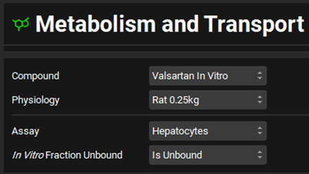
18. Now we will include the transporters kinetics in the model. Click on Metabolism and Transporter in the Modules pane located on the right-hand side of the interface.

19. Select Valsartan In vitro from the Compounds drop-down and Rat 0.25kg from the Physiology drop-down. Select Hepatocytes from the Assay drop-down and set the In Vitro Fraction Unbound to “Is Unbound”. 

20. Expand the Scaling Factors panel. Select Liver from the Tissue drop-down if not already selected and select PBPK as the Tissue Weight Source. Leave everything else as default.

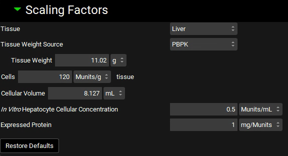
If the In Vitro Hepatocyte Cellular Concentration box appears empty, you can either click on the Restore Defaults button (as the default value is used in this tutorial) or you can type the value directly in the box.

21. Expand the Transport panel and specify the following entries in the Transporter-Specific table to convert the reported in vitro measurements ⁵ to the in vivo values in units recognized by GastroPlus®:

Transporter:                              OATP

Molecular Weight:                   76450 g/mol

Expression level:                     358 pmol/mg 

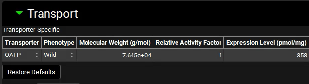
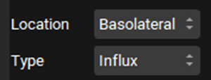
22. Select Basolateral from the Location drop-down and Influx from the Type drop-down.

Location:                                    Basolateral

Type:                                           Influx

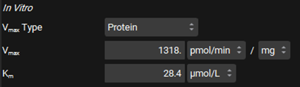
23. In the In Vitro section, leave Protein selected as the V_max Type. Switch the V_max units to pmol/min/mg and enter 1318. Leave the K_m unit as μmol/L and enter 28.4.

24. Leave Protein selected from the Clearance Type drop-down, make sure that the Clearance unit is set to μL/min/mg protein and enter 1.21.

25. The converted In Vivo values should be the same as those shown in the figure below (user inputs are marked in pink frames; the arrows mark some important parameters and outputs discussed below in more detail):

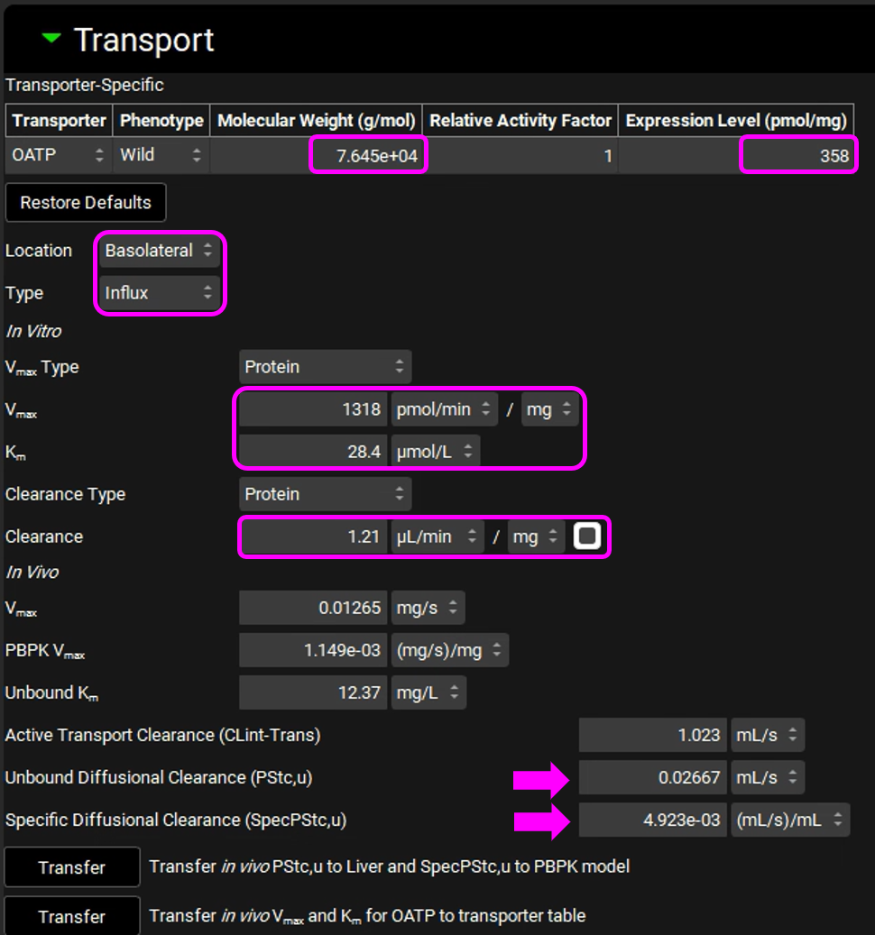
In this particular in vitro assay, the authors measured K_m and V_max values for interaction of Valsartan with the influx transporter, while also obtaining an estimate of passive diffusion. They expressed this as a diffusion rate, or permeability per mg microsomal protein. This allows us to use the same conversion factors used for K_m and V_max to obtain the in vivo diffusion rate in the entire liver. This in vivo diffusion rate corresponds to the permeability-surface area product for the liver and is shown as PStc, u (marked by the top arrow in the figure above).

We assume that the passive permeability of the drug through the membranes is the same in all tissues, with the difference in passive diffusion between the tissues caused by differences in surface areas. With that assumption, we can scale the liver PStc to other tissues by accounting for different tissue surface areas. The total cell surface areas of individual tissues are not known, so we will use tissue cell volumes as an approximation for the scaling. The total cell volume in a selected tissue is shown in the Scaling Factors panel. We use this value to calculate the PStc-per-mL-of-cell-volume, or SpecPStc,u (marked by the bottom arrow in the figure above). The SpecPStc,u value will be exported, together with all other parameters, and will be used to calculate the PStc values of individual tissues.

In these conversions, we assume that, in the liver, 2/3 of cell surface area is the basolateral membrane and 1/3 of cell surface area is the apical membrane; in kidney we assume ½ of the cell surface area for the basolateral membrane and ½ for the apical membrane.

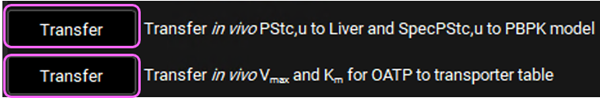
26. Click on “Transfer in vivo PStc,u to Liver and SpecPStc,u to PBPK model” and click on “Transfer in vivo V_max and K_m for OATP to transporter table”.

27. Click Done to Clear the information messages in the Message center.

28. Valsartan is cleared by biliary secretion. The kinetic parameters for the efflux transporter were not measured, so, at the moment, we will assume there is no accumulation in liver and the same kinetics as the influx transport. Adjust the following settings:

Select the MRP2 transporter in the Transporter-Specific table.

Location:      Apical

Type:             Efflux

K_m:             28.4 µmol/L

In vitro Clearance:    0 uL/min/mg (only active secretion through apical membrane).

29. The Transport panel with entries for the MRP-2 transporter is shown in the figure below (the modified entries are marked in pink frames):

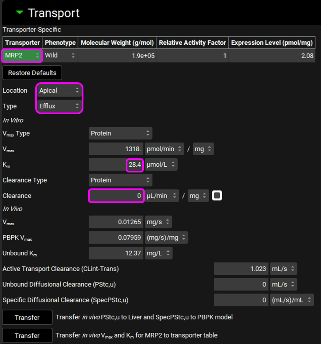
30. Click on “Transfer in vivo V_max and K_m for MRP2 to transporter table”. Click Done to clear the Information message on the Messages center.

31. Save the project and click OK.

32. We will now convert the reported in vitro human hepatocyte measurements ⁵ to in vivo values in units recognized by GastroPlus®.

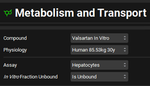
33. Select Human 85.53kg 30yo from the Physiology drop-down. Set the Assay to Hepatocytes and In vitro fraction unbound to Is Unbound.

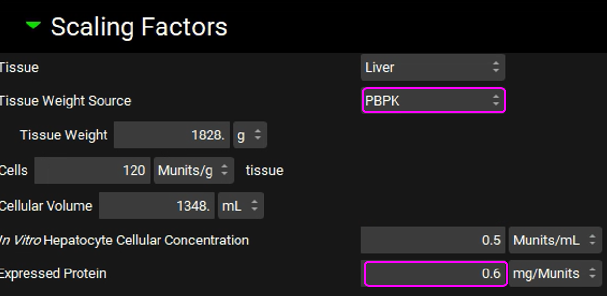
34. Expand the Scaling Factors panel and set the Tissue Weight Source to PBPK. Set the Expressed Protein to 0.6 Mg protein/Munits (The modification of this conversion factor is based on the experimental value reported in the same publication from which the in vitro data were obtained).

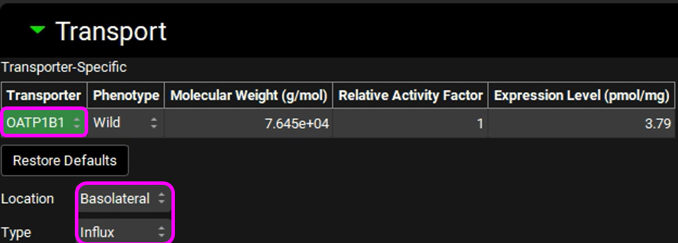
35. Expand the Transport panel and select OATP1B1 from the Transporter drop-down in the Transporter-Specific table.

36. Select Basolateral from the Location drop-down and Influx from the Type drop-down.

37. In the In Vitro section, leave Protein selected as the V_max Type. Switch the V_max units to pmol/min/mg and enter 304. Leave the Km unit as μmol/L and enter in 44.4.

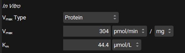
38. Leave Protein selected from the Clearance Type drop-down, Make sure that the Clearance unit is set to μL/min/mg protein and enter 0.724.

39. The converted In Vivo values should be the same as those shown in the figure below (user inputs are marked in pink frames):

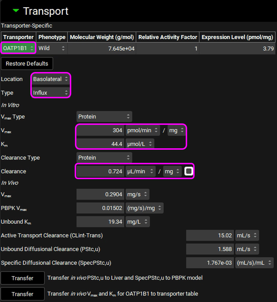
40. Click on “Transfer in vivo PStc,u to Liver and SpecPStc,u to PBPK model” and click on “Transfer in vivo V_max and K_m for OATP1B1 to transporter table”. Click Done to clear the information message on the Messages Center.

41. Similarly to the rat simulations, we will make an assumption of the same kinetics for MRP2 as for OATP1B1. Adjust the following settings:

Select MRP2 from the Transporter drop-down in the Transporter-Specific table.

Location:      Apical

Type:             Efflux

K_m:             44.4 µmol/L

In vitro Clearance:    0 uL/min/mg (only active secretion through the apical membrane)

42. The entries for the MRP2 transporter are shown in the figure below (the modified entries are marked in pink frames):

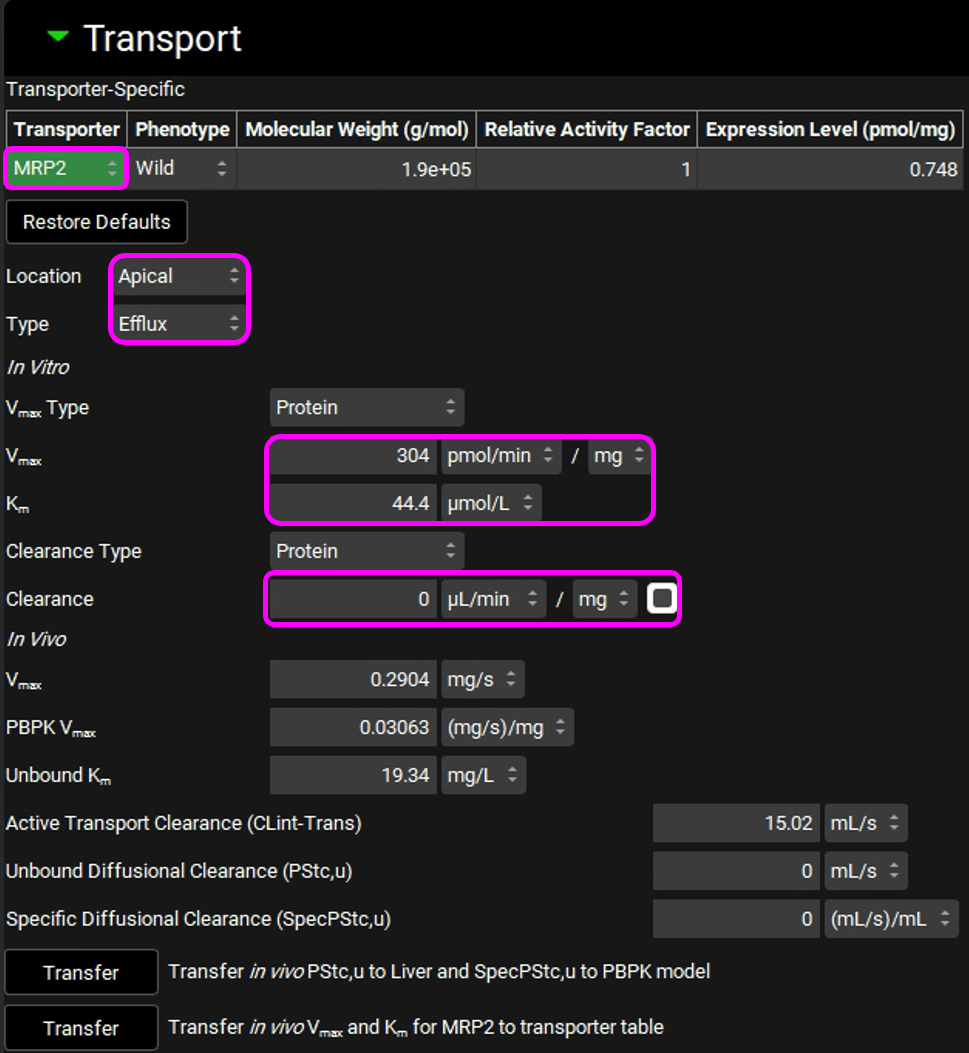
43. Click on “Transfer in vivo V_max and K_m for MRP2 to transporter table”. Click Done to clear the Information message on the Messages center.

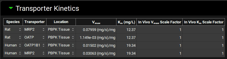
44. Navigate to the Compounds view to see the transferred values in the Transporter Kinetics panel.

45. Save the project and click OK.

46. Navigate to the Pharmacokinetics view. Make sure that Valsartan In Vitro is selected from the Compound drop-down and Rat 0.25kg from the Physiology drop-down. Open the PBPKPlus™ panel by clicking on the green arrow or double clicking on the panel header. Since Valsartan undergoes an active uptake transport, we will need to set the liver tissue to “permeability limited”. 

47. Click on the Liver tissue on the PBPK diagram. You can change the tissue type by right clicking on the tissue or by switching the “Tissue Type” drop-down to Permeability Limited in the Compound sub-panel on the right-hand side.

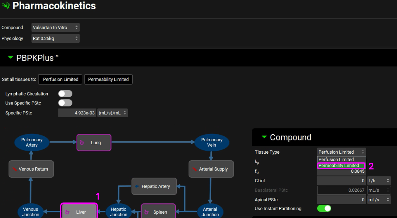
48. Click Done to Clear the message in the Messages center about recalculating Tissue Kps.

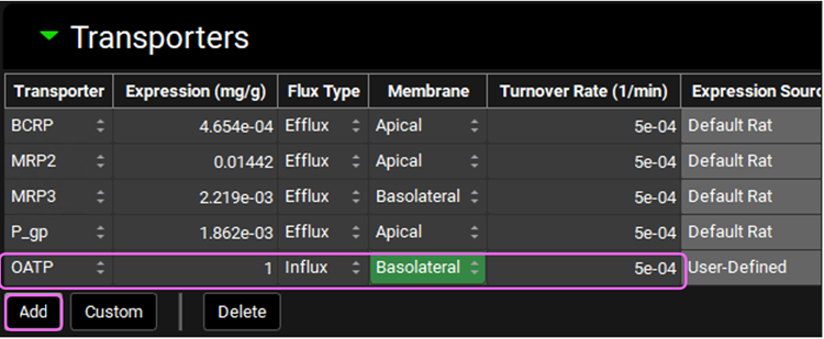
49. Having the Liver tissue still selected, scroll down to the Transporters sub-panel on the right-hand side. Click on “Add” to include the OATP transporter to the Liver. Select OATP from the Transporter drop-down, set the Expression to 1mg/g, Membrane to “Basolateral”, Flux Type to “Influx”, and Turnover Rate to 5e-04 1/min.

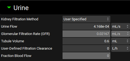
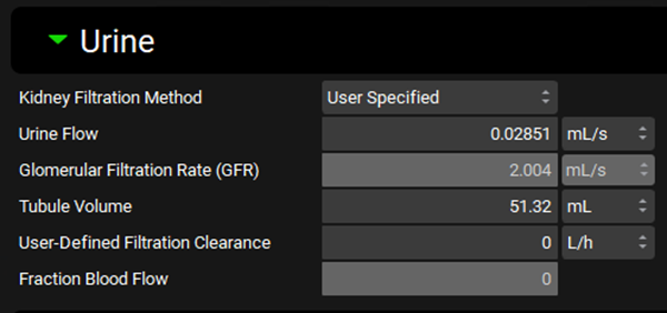
50. Since Valsartan is cleared by biliary secretion, we will set the kidney clearance to zero. Click on the Kidney tissue on the PBPK diagram and scroll to the Urine sub-panel on the right-hand side of the diagram. Set the Kidney Filtration Method to “User Specified”. Note that the User-Defined Filtration Clearance is set to 0 L/h (value can be edited but will be left as 0 for this example).

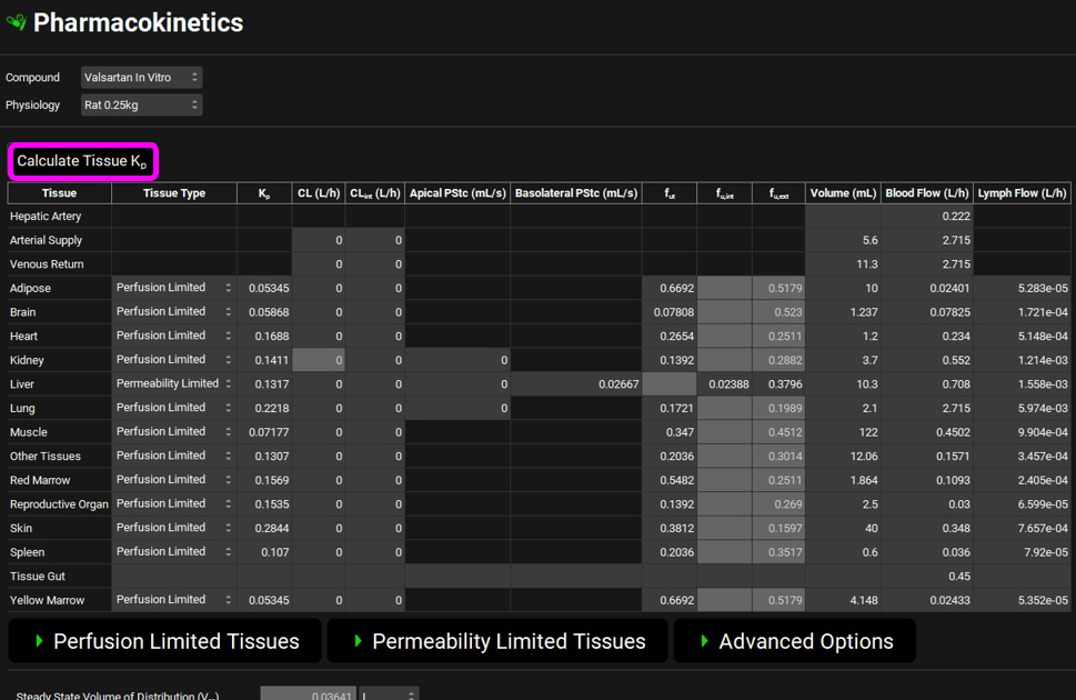
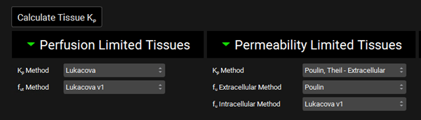
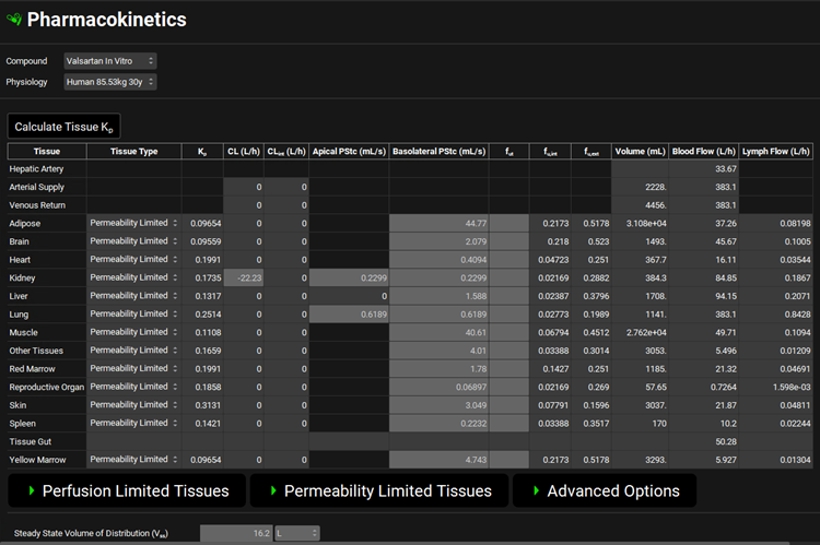
51. Scroll down to the PBPK table located below the PBPK diagram. Expand the Perfusion Limited Tissues and Permeability Limited Tissues located at the bottom of the table. Set the Kp calculation methods and fraction unbound in tissue as shown in the figure below.

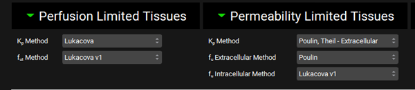
52. Scroll up to the top of the PBPK table and click the Calculate Tissue Kp button (the Liver tissue was changed to a permeability-limited tissue, and we need to recalculate the proper Kp for that type of tissue model).

53. Navigate to the Simulations View in the navigation pane and select the Rat IV 0.25mg simulation.

54. Expand the Drug Administration panel and select Valsartan In Vitro from the Compound drop-down and 0.25mg IV bolus from the Dose Schedule drop-down. Select the Rat 0.25kg schedule from the Physiology Schedule drop-down and set the Pharmacokinetic Model to PBPK.

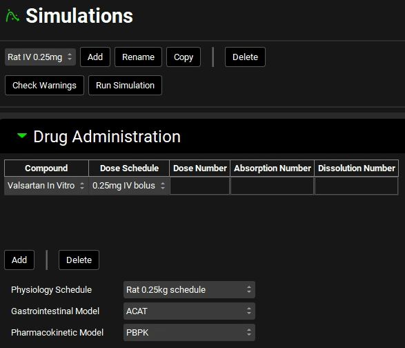
55. Click Done to Clear the information messages in the Message center.

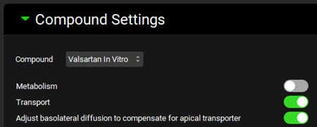
56. Expand the Compound Settings panel and select the Transporter toggle on, if not already selected.

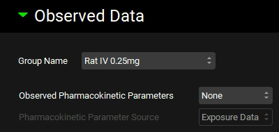
57. Scroll down to the Observed Data sub-panel and select Rat IV 0.25mg from the Group Name drop-down.

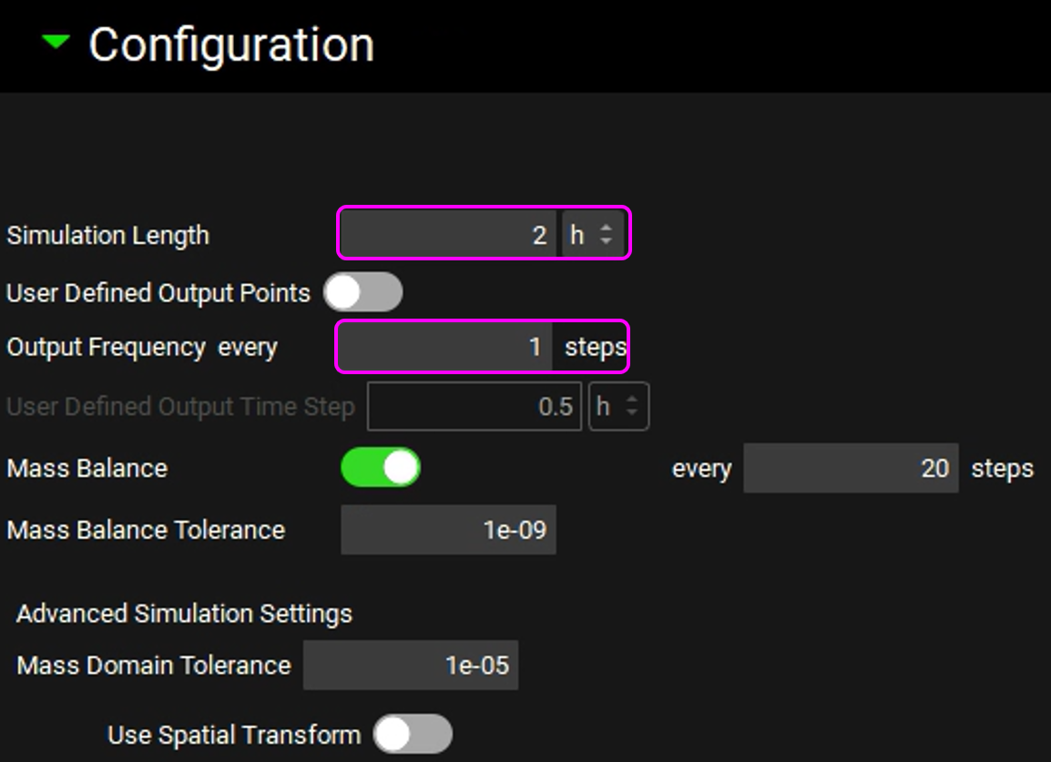
58. Expand the Configuration panel to set the simulation length to 2h and the Output Frequency to every 1 steps.

59. Save the project and click OK.

60. Click on Check Warnings and then Run Simulation. The results will be displayed in the Analysis view.

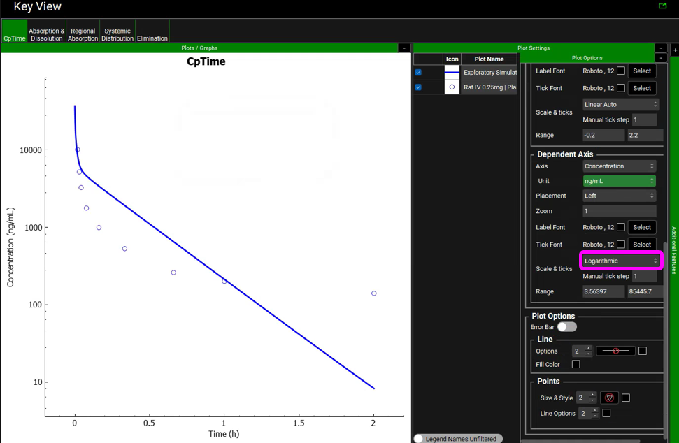
61. In the Key View set the Concentration axis to be in Log scale for the C_p Time plot. Click on the “+” on top of the Plot Settings bar and then click on the “+” on top of the Plot Options bar. Scroll down to the Dependent Axis frame and select Logarithmic for Scale & ticks.

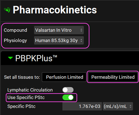
The usual approach to dealing with this type of mismatch between the simulation and observed data includes modification of the transporter’s V_max value. However, we will try a different approach. Let’s assume that if the drug has low passive permeability in the liver, it will have low passive permeability in all tissues. We will change all tissues to permeability-limited tissue models and use the Specific PStc (PStc per mL of cell volume) to calculate the PStc values for all tissues.

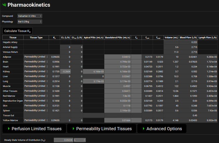
62. Navigate to the Pharmacokinetics view in the Navigation Pane. Make sure that Valsartan In Vitro and Rat 0.25kg are selected. Set all tissues to Permeability limited and click on the Use Specific PStc toggle.

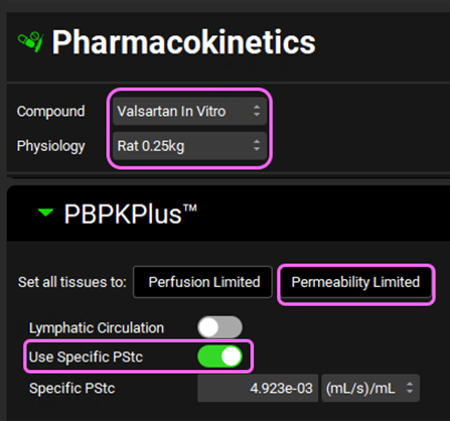
63. Individual tissue PStcs will be automatically calculated from the SpecPstc parameter (which we obtained earlier from the in vitro data) and the individual tissue cell volumes (calculated from the total volume and extracellular water fraction for each tissue).

64. Scroll down to the PBPK table located below the PBPK diagram and click on Calculate Tissue Kp to recalculate the Kp relevant for all permeability-limited tissues. Click Done to Clear the information messages in the Message center.

65. Save the project and click OK.

66. Click on the Simulations view and run the Rat IV 0.25mg simulations again. Examine the results in semi-log scale in the Analysis view:

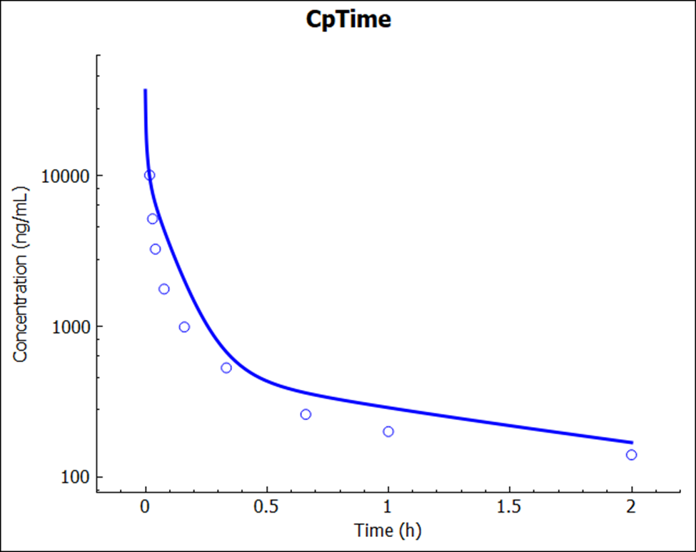
Notice that there is an excellent match between the predicted and experimental C_p-time profile. This simulation result was a pure prediction, generated without the need for any empirical scaling factors.

PART 2 – Human predictions 

1. Now let’s try the same prediction for humans. Navigate to the Physiologies view in the navigation pane and select Human 85.53kg 30y from the Physiology drop-down.

2. Navigate to the Pharmacokinetics view and set all tissues to Permeability limited. Select the Use Specific PStc toggle. Make sure Valsartan In vitro and Human 85.53kg 30y physiology are selected. Click Done to Clear the information messages in the Message center.

3. Since Valsartan is cleared by biliary secretion, we will set the kidney clearance to zero. Click on the Kidney tissue in the PBPK diagram and scroll down to the Urine panel on the right-hand side of the diagram. Select Kidney Filtration Method to User Specified.

4. Scroll down to the PBPK table located below the PBPK diagram. Set the Kp calculation methods and fraction unbound in tissue as shown in the figure below. Click the Calculate Tissue Kp button to recalculate the Kps relevant for permeability-limited tissues.

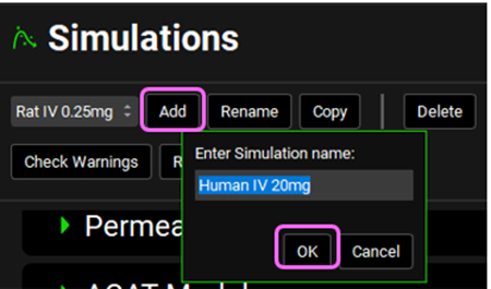
5. Navigate to the Simulations view and click Add to create a new simulation. Name it “Human IV 20mg” and then click OK (or press enter).

6. Expand the Drug Administration panel and select Valsartan In Vitro from the Compounds drop-down. Select 20mg IV bolus from the Dose Schedule drop-down. Select Human 83.53kg 30y schedule from the Physiology Schedule drop-down and set the Pharmacokinetic model to PBPK. Click Done to Clear the information messages in the Message center.

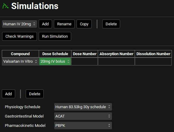
7. Expand the Compound Settings panel and select the Transporter toggle if not already selected.

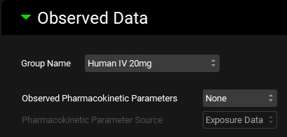
8. Scroll down to the Observed Data sub-panel and select Human IV 20mg from the Group Name drop-down.

9. Expand the Configuration panel to set the simulation length to 24h and the Output Frequency to every 1 steps.

10. Click on Check Warnings and then Run Simulation. The results will be displayed in the Analysis view. Switch to a semi-log scale for better visualization.

Notice a very reasonable prediction (no empirical scaling factors were used or adjusted) of Valsartan exposure after intravenous administration in human.

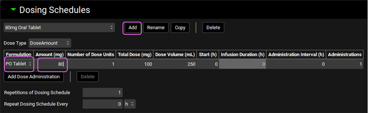
11. Finally, let’s verify the human PK by simulating the oral administration. Click on the Dosing view in the navigation pane. Expand the Formulations panel and select the PO Tablet formulation. The default selections already reflect an oral tablet, hence we will leave it as is.

12. Expand the Dosing Schedules panel and click on Add to create a new schedule. Name it “80mg Oral Tablet” and click OK. Select the PO tablet Formulation and set the Amount (mg) to 80mg.

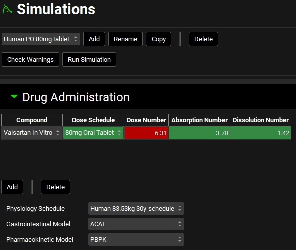
13. Click on the Simulations view in the navigation pane. With the “Human IV 20mg” selected, click on Copy, naming it Human PO 80mg tablet. Change the Dose Schedule to 80mg Oral Tablet.

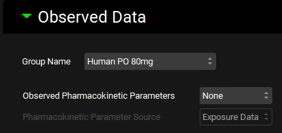
14. Expand the Observed Data sub-panel under the Compound Setting panel and select Human PO 80mg from the Group Name drop-down.

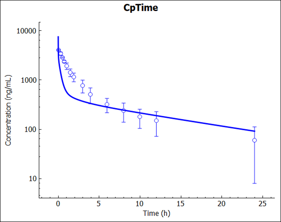
15. Save the project and click OK. Click on Check Warnings and then Run Simulation.

16. The prediction (no empirical scaling factors were used or adjusted) again resulted in a very reasonable match to the reported C_p-time profile.

The PO dose may need to include the MRP2 effect along the intestine, which was not incorporated in this tutorial.

You may have also noticed that for this specific tutorial, we are using the older method for the calculation of intracellular unbound fraction: “Fu Int: Lukacova v1”. Analysis of the rat PK data showed that the shape of the C_p-time profile is captured better with the lower fraction unbound in different tissues as predicted with this approach. We do not have a mechanistic explanation for this drug behavior yet and, for now, would simply use the same strategy as when deciding on what is the best approach to predict CL or Kps in human – i.e., utilize animal PK data to build and validate the PBPK model, and work with the same types of inputs and methods/mechanisms when predicting first-in-human exposure.