Tutorial: Observed Data

Observed Data can contain data that may be used as inputs into Simulations or data which can be used to visually compare GastroPlus® predictions or to fit GastroPlus® models.

Observed Data Types are as follows: Chemical Degradation Rate, Dissolution Rate (Z Factor), Exposure Data, Immune Cell Layer Thickness, In Vitro Dissolution Release, In Vivo Controlled Release, Inflammation, Particle Size Distribution, Pharmacodynamic Effect, Precipitation Time, and Solubility.

In this tutorial we will look at entering and using the Solubility Observed Data Type. Entering and using Exposure Data is covered in the GPX™ Run Modes and Loading Observed Data tutorial and the PBPKPlus™ Module Tutorial. Entering and using Pharmacodynamic Effect Data is covered in the PDPlus™ Module Tutorial. Using In Vitro Dissolution Release data is covered in the IVIVCPlus™ Module Tutorial.

In this tutorial, we will cover:

• Opening the GPX™ project and familiarization with the assets

• Loading Solubility versus pH data and updating experimental parameters

• Utilizing the Observed Solubility vs pH data in Simulations

Opening the GPX™ project and familiarization with the assets

1. Open GPX™ and, in the Dashboard view, click on the icon next to Select to open an Existing project.

2. Click Browse and navigate to the C:\Users\<user>\AppData\Local\Simulations Plus, Inc\GastroPlus\10.2\Tutorials\Observed Data Tutorial - Miconazole folder and select the project file Observed Data Tutorial - Miconazole.gpproject by clicking on it and clicking Open.

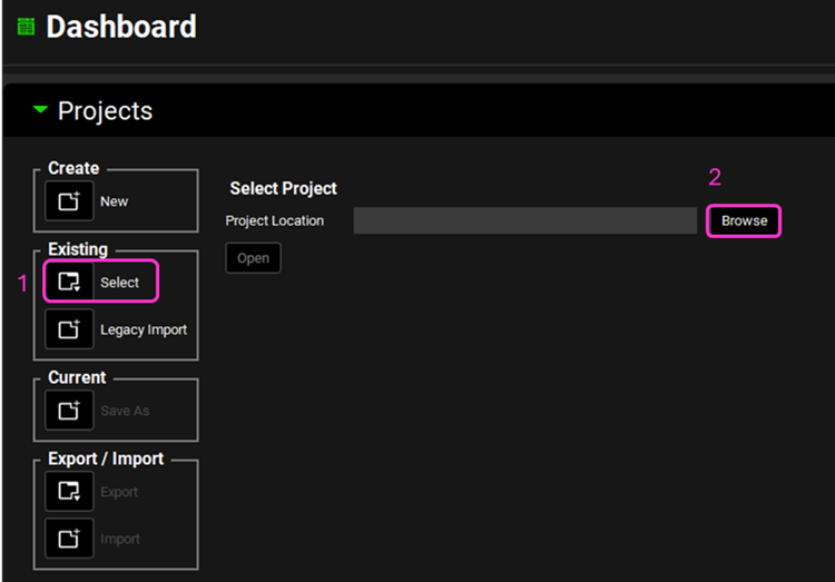
3. Save a copy of the project by clicking on the icon next to Save As, entering “Observed Data Tutorial Miconazole complete” as the Project Name and click Browse to navigate to/add a folder to Save the project in. Click Save - you will see an information message in the Messages Center indicating that the project has been successfully copied. This message will disappear once you click 'Yes' on the pop-up window that also appears. Note that the name of the project visible in the top right corner of the interface is the one that has just been created.

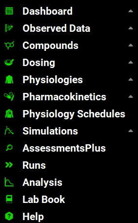
4. Move through the views on the navigation pane from Compounds to Simulations, observing the information that has been entered in this project.

The project contains one compound, Miconazole, that has been imported using ADMET Predictor^®, with a 500 mg IR tablet dose schedule, a 30y 70kg American male physiology and a compartmental PK model. The general clearance has been updated from the ADMET Predictor^® value to 0.65 L/h/kg.

Loading Solubility versus pH data and updating experimental parameters

Once the solubility versus pH data is entered, an interpolated or a theoretical solubility model can be used in a simulation. The solubility versus pH data can be fitted in order to adjust pKa and solubility factor values. We will create three simulations that use interpolated or theoretical solubility models and non-fitted or fitted pKa and solubility factor values.

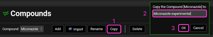
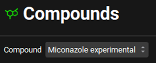
1. Create a copy of the compound – this will allow you to add experimental values without overwriting the ADMET Predictor^® properties. Navigate to the Compounds view and click Copy, name the compound “Miconazole experimental” and click OK (or press Enter).

2. Save the project using the Save button in the top right corner of the interface and click OK on the Save completed message.

3. To add solubility versus pH data:

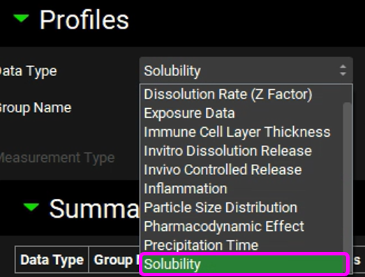
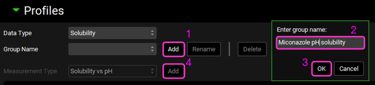
Navigate to the Observed Data view and select Solubility as the Data Type by clicking in the box containing “Exposure Data” and choosing Solubility from the drop-down list.

4. Click “Add” next to the Group Name and type “Miconazole pH solubility” in the pop-up box for the group name then click OK.

5. Ensure the Measurement Type is Solubility vs pH and click “Add” then type “sol vs pH” in the pop-up box for the Enter series name and click OK.

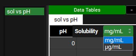
6. Check the correct units are displayed in the Solubility (mg/mL) column of the data table. To change the units, click on the unit in the column header and select the appropriate one from the list.

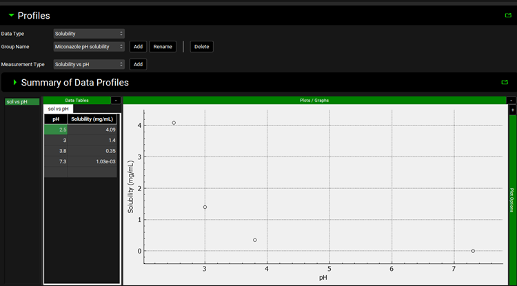
7. Open the Input Data for Observed data tutorial.xlsx and copy the Miconazole solubility data found on the Miconazole solubility tab. Move to GPX™ and paste the data by right clicking in the first cell of the pH column and selecting Paste. The plot should be enabled displaying the observed data.

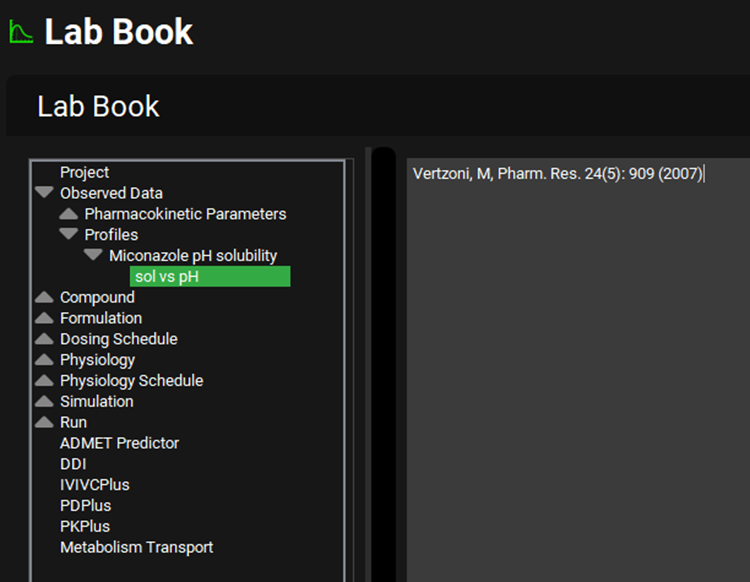
8. Navigate to the Lab Book view and expand the Observed Data section by clicking on the grey arrow. Expand the Profiles section and then the Miconazole pH solubility section in the same way. Click on the sol vs pH line, move to the Input Data for Observed data tutorial.xlsx, copy the reference from which the data was obtained and paste into the free text section of the Lab Book by right clicking and selecting paste.

9. Save the project and click OK.

10. To update selected compound properties with experimental data, navigate to the Compounds view and ensure that compound selected is “Miconazole experimental”.

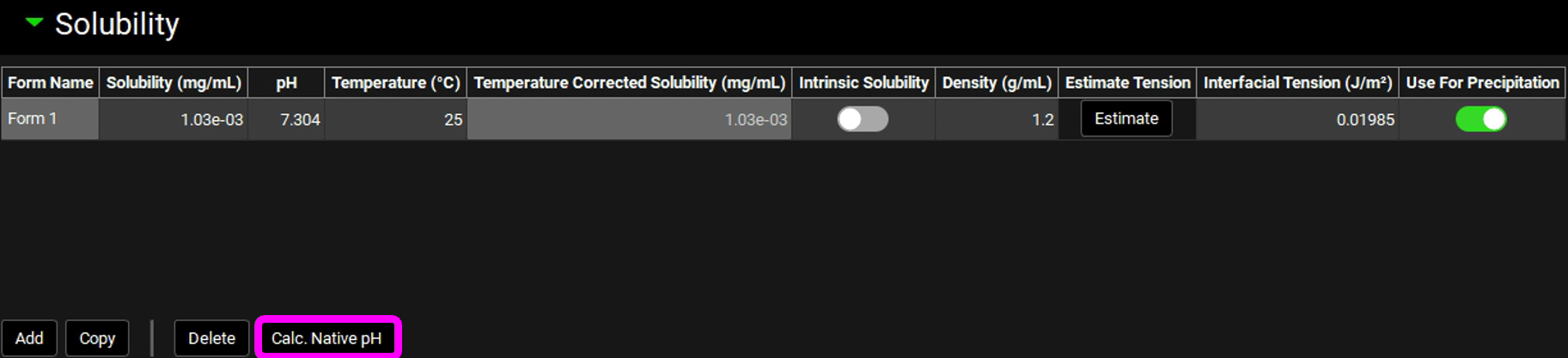
11. Expand the Solubility panel by clicking on the green arrow or double clicking on the Solubility panel header bar.

12. Click in the Solubility (mg/mL) cell and (if necessary, the entire number can be selected by holding Ctrl and pressing A) type in the experimental solubility of 0.00103 mg/mL and press Enter.

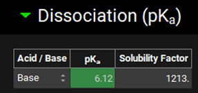
13. Minimize the Solubility section (by clicking on the green arrow or double clicking on the Solubility panel header bar) and expand the Dissociation (pKa) panel in the same way.

14. Update the pKa from 6.358 to 6.12. It is interesting to note how closely ADMET Predictor^® estimated this property. A Warning message is displayed in the Messages Center prompting the user to recalculate the tissue Kps if a PBPK model is being used. As we are using a compartmental PK model, the message can be cleared by clicking Done.

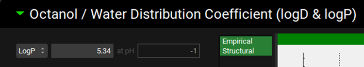
15. Minimize the Dissociation (pKa) panel and expand the Octanol / Water Distribution Coefficient (logD & logP) panel and update the LogP from 5.714 to 5.34 ¹ by typing in the value and clicking elsewhere. A re-calculate Kp message is displayed in the Messages Center and can be cleared by clicking Done.

16. Return to the Solubility panel, expand it and Click the Calc. Native pH button, this calculates the pH of a solution at a concentration of 0.00103 mg/mL.

17. Save the project and click OK.

Utilizing the Observed Solubility vs pH data in Simulations

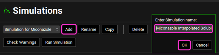
1. Navigate to the Simulations view, click the Add button and name the Simulation “Miconazole Interpolated Solubility”. Click OK.

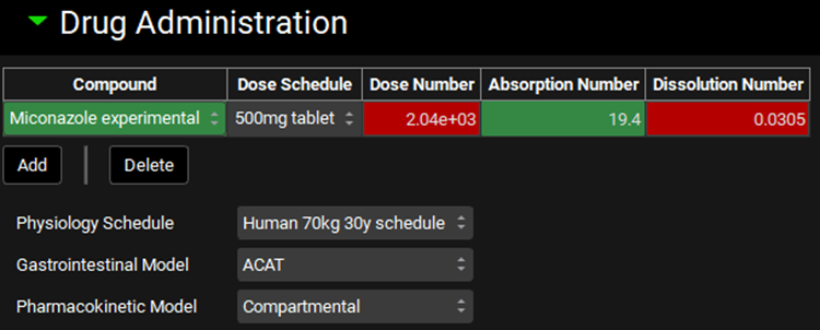
2. Expand the Drug Administration panel and select the compound “Miconazole Experimental”.

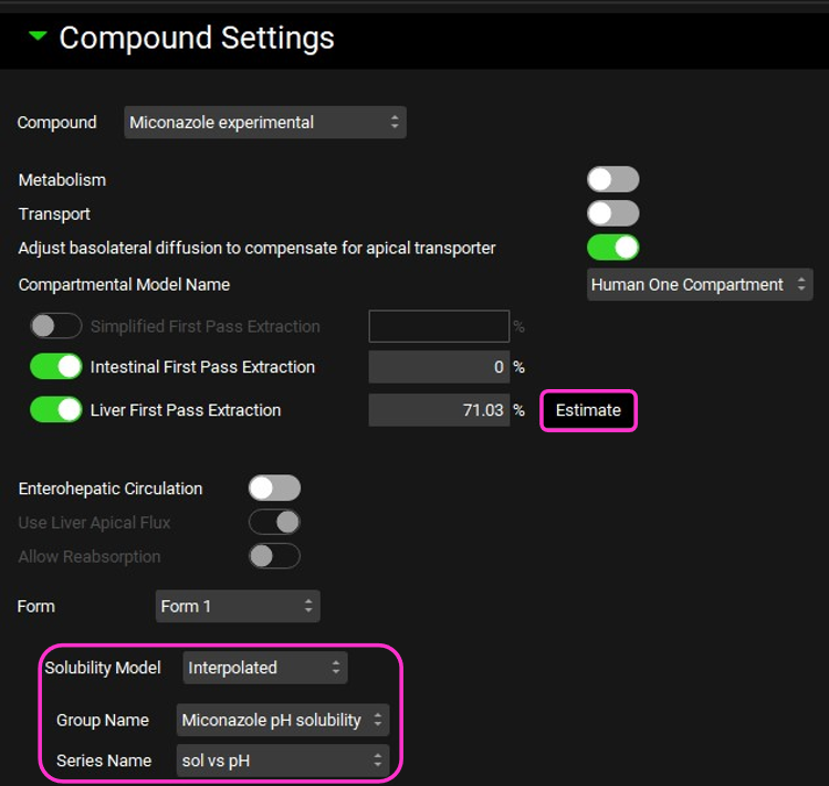
3. In the Compound Settings panel, change the Solubility Model from Theoretical to Interpolated. As the project only has one solubility vs pH data set, the miconazole one is automatically selected.
   

This will use the entered data with linear interpolation – this method is not generally recommended as it is not the way solubility-pH dependence behaves. The smooth interpolation provided by the theoretical pKa model, as fitted to the data, is more realistic.

4. Click on Estimate to enable the Liver First Pass Extraction to be calculated.

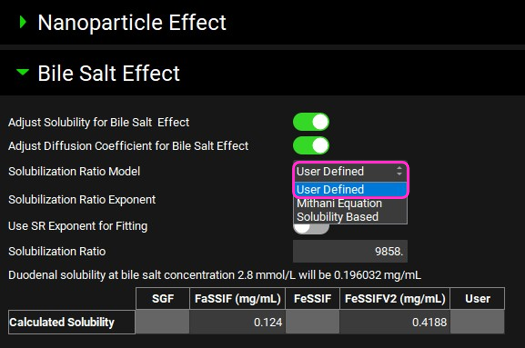
5. Expand the Bile Salt Effect sub-panel under Compound Settings panel. Click in the box containing Solubility Based and switch the Solubilization Ratio Model to User Defined.

6. Save the project and click OK.

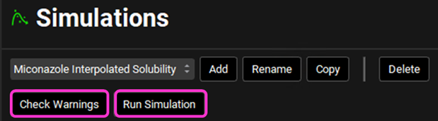
7. Click on the Check Warnings button (located at the top of the view underneath the Simulations selection area) and then on the Run Simulation button.

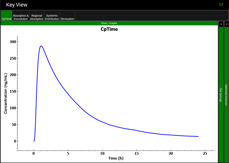
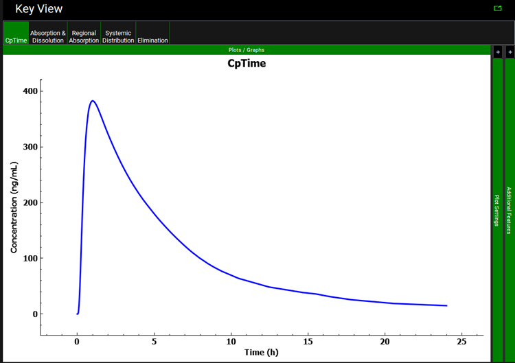
8. A single simulation has now been run and when it completes it will automatically switch to the Analysis view, displaying the last Key View plot viewed. If necessary, switch to view the C_p-Time plot.

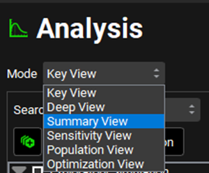
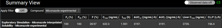
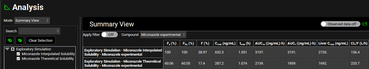
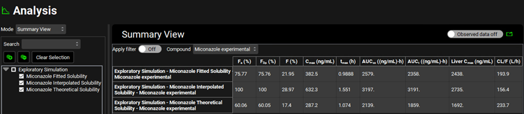
9. Select the Summary View as the Mode and use the Observed data on toggle to turn the Observed data off (the toggle will turn grey).

10. Notice the fraction absorbed is 100%. This value is much higher than is observed experimentally.

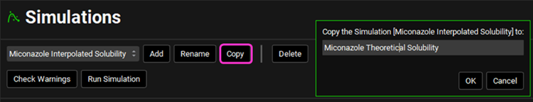
11. Go to the Simulations view. Copy the “Miconazole Interpolated Solubility” Simulation by clicking the Copy button next to the name and replace “Interpolated” with “Theoretical” and click OK.

12. Select the Theoretical Solubility Model in the Compound Settings panel.

13. Click on the Check Warnings and then on the Run Simulation button.

14. A single simulation has now been run and when it completes it will automatically switch to the Analysis view, displaying the C_p-Time Key View plot.

15. Select the Summary View as the Mode and check the box next to the “Miconazole Interpolated Solubility” in the simulation tree to add the results of the initial simulation to the summary table. Observe that using the Theoretical Solubility profile decreases the F_a to approximately 60%.

16. Navigate to the Compounds view and expand the Dissociation (pKa) panel. Select the observed data profile by clicking in the box next to the Group Name and selecting “Miconazole pH solubility”.

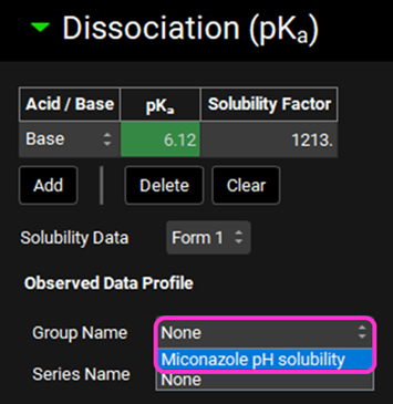
17. The plot should update to display the observed data points along with a curve describing the current model. The curve does not reflect the observed data with the predicted solubility at low pH being lower than observed.

18. Turn the toggle named Enable pKa Fitting on by clicking on it, the toggle should turn green.

19. Click the Fit button, an additional, green, line appears on the plot describing the fitted curve.

20. If the fit is acceptable and describes the observed data, click Accept Fit. The blue line indicating the original theoretical curve will clear and the newly fitted line will go from green to blue.

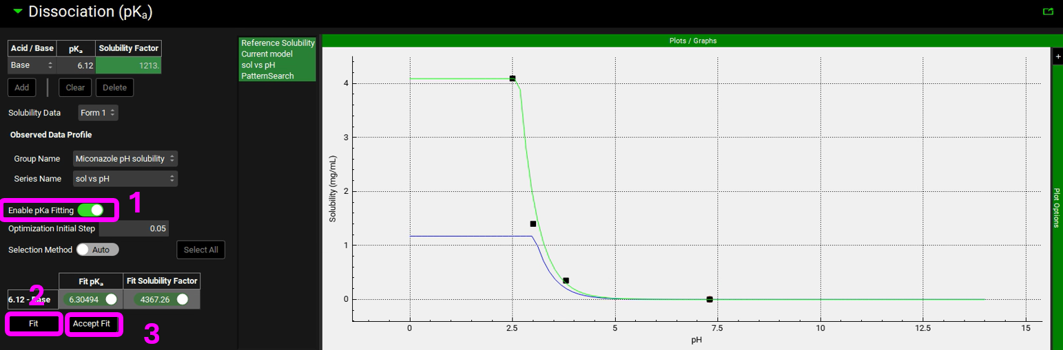
NB – numbers reflect the order of the steps in the screenshot, rather than corresponding to the steps in the tutorial.

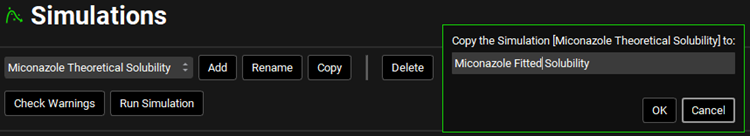
21. Navigate back to the Simulations view and copy the “Miconazole Theoretical Solubility” simulation, naming the new Simulation “Miconazole Fitted Solubility” and click OK.

22. Save the Project and click OK.

24. Click on the Check Warnings and then on the Run Simulation button.

25. A single simulation has now been run and when it completes it will automatically switch to the Analysis view, displaying the C_p-Time Key View plot.

26. Select the Summary View as the Mode and check the box next to Miconazole Interpolated Solubility and Miconazole Theoretical Solubility in the simulation tree to add the results of the initial simulation to the summary table. Observe that using the Fitted Solubility profile results in a F_a of approximately 76%.

Note that if you rerun the Theoretical simulation at this point it will give identical results to the Fitted simulation we have just run because the fitted solubility vs pH curve has replaced the one we used in the original simulation. If you wish to keep the original theoretical solubility vs pH curve then you should copy the compound prior to fitting in step 18.

27. Return to the Key View Mode and uncheck the Miconazole Theoretical Solubility simulation. Expand the Additional Features pane by clicking on the “+”. Click on the dropdown box containing “Tissue” to activate the Color by drop-down list. Select “Random” and click the Color by: button to activate this setting in the plot (NB the colors you get may be different to the screenshot – repeatedly clicking the Color by: button cycles through different color options). To identify which curve represents which simulation, click the “-” next to Additional Features and expand the Plot Settings pane by clicking on the “+” then hover over the plot name to display the complete text.

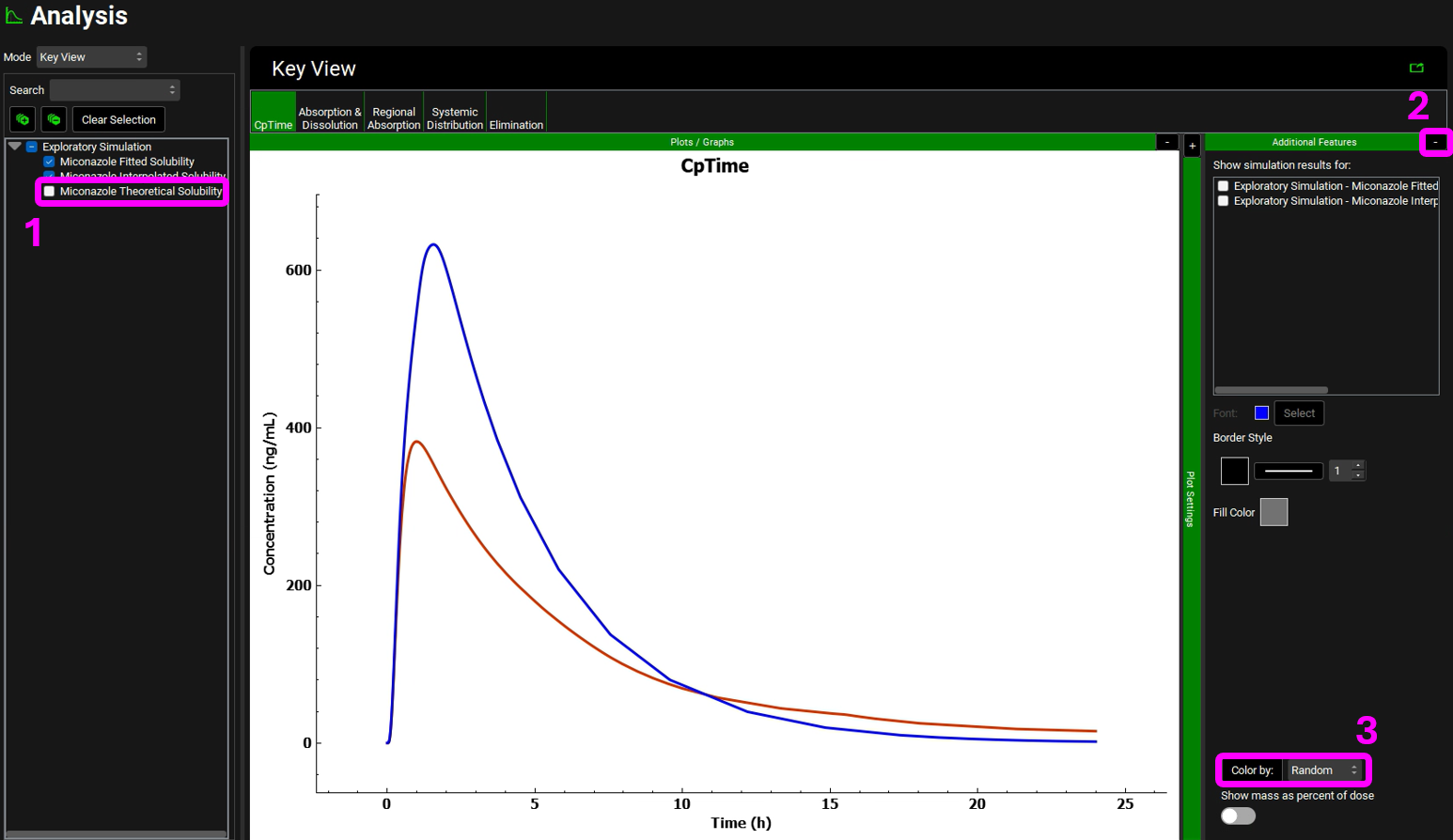
NB – numbers reflect the order of the steps in the screenshot, rather than corresponding to the steps in the tutorial

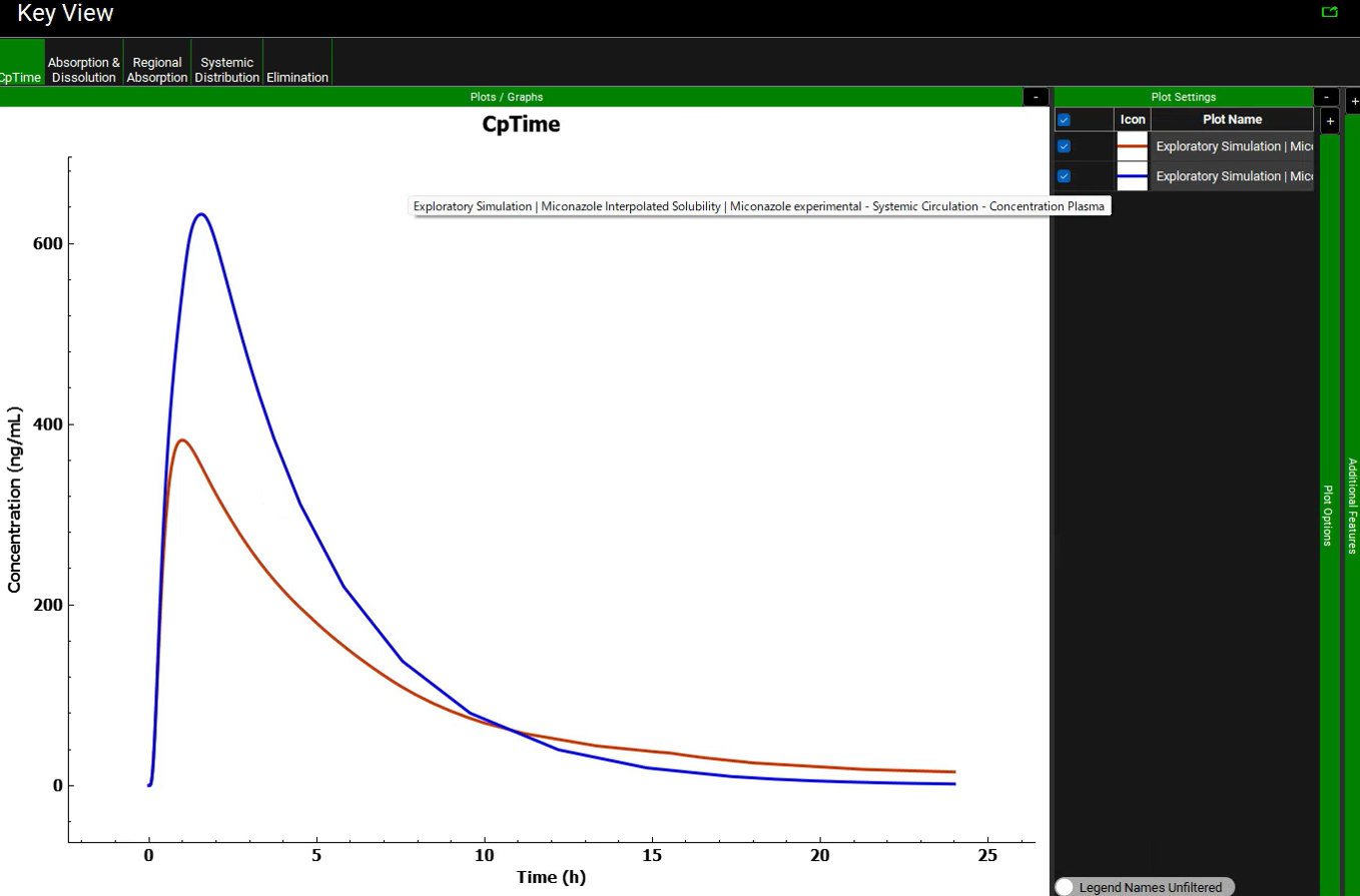
The brown curve uses the fitted solubility curve while the blue curve uses the interpolated curve. The large difference is due to the interpolation between the third and fourth data points. Linear interpolation calculates solubility that is too high in the pH range of duodenum and jejunum for the human fasted physiology (6.0-6.4).